LLM Inference Economics from First Principles


The main product LLM companies offer these days is access to their models via an API, and the key question that will determine the profitability they can enjoy is the inference cost structure. In this text we will explain where the cost of serving/hosting LLMs comes from, how many tokens can be produced by a GPU, and why this is the case. We will build a (simplified) world model of LLM inference arithmetics, based on the popular open-source model-LLama 3.3. The goal is to develop an accurate intuition regarding LLM inference.
The topic of LLM inference economics has far-reaching implications beyond technical considerations. As AI capabilities rapidly advance, inference efficiency directly shapes both industry economics and accessibility. For AI labs, token production costs fundamentally determine profit margins and the cost of generating synthetic training data-more efficient inference means higher returns on a fixed investment in hardware that can fuel further research and development cycles. For users, lower token costs democratize access to these powerful tools, potentially transforming AI from a premium resource into an everyday utility available for even routine tasks. Understanding these cost structures isn't merely academic-it provides insight into one of the key economic forces that will shape AI development in the coming years as we approach increasingly capable systems.
The primary cost behind a generated token boils down to the cost of compute - you need to buy or rent a GPU. In both cases, there is a fixed cost associated with running a GPU per hour. Each GPU can produce a limited number of tokens in an hour. The number of tokens produced per hour divided by the cost of hardware per hour will tell you the unit cost of generating a single token. This is how most of the LLM providers price their API offerings, and this will be the model we will explore.
Model parameters and hardware requirements
As a basis for our inference economics analysis, we will use LLama 3.3 70B. Even today it is still one of the most popular open-source models and an architecture around which a big portion of the industry standardized. There are numerous model fine-tunes of the Llama weights, and while these models will produce different outputs, because they share the same model architecture, they require exactly the same compute resources to run them. Hence, we consider Llama a good candidate to provide a real-world example that will be representative but, at the same time, quite simple to grasp.
LLMs store their "knowledge" in parameters-essentially the weights that define the model's behavior. These parameters require memory to store and compute resources to process. Generally, the more parameters a model has, the greater its resource demands, but so are its potential capability on downstream tasks. Llama 3.3 70B has around 70 billion parameters, which is where its name comes from.
A so-called decoder-only transformer model, like Llama, usually consists of the following components:
one input embedding layer-converting tokens, or words, into vector representations.
multiple transformer layers, each layer containing some parameters for the self-attention part and some for the MLP part.
language modeling (LM) head-the final layer
We assume the reader has a basic understanding of these concepts; hence, we will not be providing the deep intuitions behind them. If you are unfamiliar with the transformer architecture, please stop here and check out one of these amazing tutorials.


Now, let's break down the model's parameter count step by step, verifying that the claimed 70 billion parameters hold up. To do so, let’s start by looking at the Llama model config in Fig. 1. We can see there are multiple keys and values. Keys, such as hidden_size informing us about the sizes of specific parts of the model. We can use them to calculate the total model size. To grasp the high-level overview of the architecture, take a look at Fig. 2. You can see all three parts we described above, and the graph also shows some implementation details that we will dive into in the next section.
For input embedding layer, we need to convert every possible token position into its vector representation. Hence we have:
parameters.
Then we have N transformer layers (see Fig. 2). Each of these layers has typically many millions parameters that we will need to store in memory in order to run the model. Their sizes can be calculated with hyper parameters from the config.json above:
*The w_v and w_k being 1/8th the size of the w_q is something Llama architecture specific. This is due to the Llama team using a technique called Group Query Attention in which the model has fewer K and V heads than the total attention heads. You can verify this by looking at num_key_value_heads in the hyperparameters from the model config. The model intermediate_size being 3.5x the hidden size is as well a Llama architecture-specific value. These were chosen by the Llama team, and we take them at face value, also to simplify our calculations.
Bringing us to a total of
per transformer block.
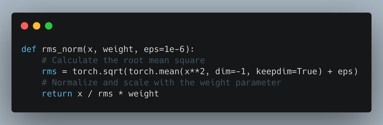
Finally, we apply a last RMS Norm before feeding the representation into the LM head, which converts vectors into token logits.
Summing up all of these parameters we obtain:
We can find the values of each of these, vocab_size , hidden_size , num_hidden_layers in the config in Fig. 1. Substituting these values into the equation we will get:
Each parameter is a floating-point number in a bfloat16 format-e.g., 0.22312, -4.3131. Storing each of these numbers takes 16 bits which is 2 bytes of memory. Given that we have a total of 70,553,706,496 parameters to store, we will need 141,107,412,992 bytes or 141GB just to store the model weights in GPU memory.
Note that 141GB is more memory than there is on the most common data center GPUs, such as the Nvidia A100 or H100. Each of these GPUs comes with only 80GB of total memory (we refer to this memory interchangeably as HBM, high bandwidth memory, or global memory). Hence, for serving models, we usually use multiple cards for a single instance of a model. In practice, for more optimal model serving, we want to use more, 4 or even 8 such GPUs. Let’s now just take it at face value, and we will elaborate on why this is the case in the later part of this text.
Compute and memory bound
When looking at the specification of a GPU, you should be paying most attention to two metrics:
Compute: measured in FLOPS - how many floating-point operations (addition and multiplication) a GPU can do in a second*.
Memory bandwidth: how many bytes can be loaded from the global memory in a second.
These two factors dictate how quickly you can process computations; they affect the speed of a single feedforward operation and determine the generation speed (measured in tokens per second, tps) and ultimately define your cost per token.
* Please be aware that FLOPS and FLOPs mean different things. FLOPs (small s) is the plural of floating-point operations not considering time at all but FLOPS (capital S) means floating-point operations that happen within a second

A computer program (such as running an LLM) can be characterized by its arithmetic intensity. Arithmetic intensity is a concept that describes the ratio of computational operations, such as addition or multiplication (measured in FLOPs), to memory accesses (measured in bytes). A higher arithmetic intensity indicates that the program performs more computations per unit of data fetched from memory, which typically leads to better utilization of the processor's computational capabilities and reduced bottlenecking on memory bandwidth. LLM inference has a very low compute intensity because it involves repeatedly accessing large model weights from memory with relatively few computations per byte fetched.
For A100:
FLOPS: 3.12 * 10^14 floating point operations can be performed in a per second
Memory: 2.03 * 10^12 bytes can be loaded from global memory (HBM) per a second
For H100:
FLOPS: 9.89 * 10^14 floating point operations can be performed in a per second
Memory: 3.35 * 10^12 bytes can be loaded from global memory (HBM) per a second
As you'll see in the next parts of this text, LLM inference has both a phase that's heavily compute-bound (very high arithmetic intensity) and a heavily memory-bound (very low arithmetic intensity). The majority of the wall clock time is spent in the memory-bound phase, so the goal of efficient LLM inference is to maximize the utilization of the GPUs' compute capacity during the memory-bound phase. So increasing the arithmetic intensity for the memory-bound phase represents a fundamental optimization target that directly translates to improved inference economics.
In the context of LLMs, in order to generate a token, we need to load the entire model with all parameters from global memory (HBM) (we utilize the memory bandwidth) and calculate the intermediate activations (we use the compute). The ratio between compute and memory utilization is crucial in determining what can be optimized and how to enjoy better inference economics. In the next part we will go more in depth on the two phases of LLM inference:
prompt processing or so called pre-fill phase
token-by-token or so called decoding phase
The end-to-end latency of an LLM request depends critically on the efficiency of both these two phases.
FLOPs in matrix multiplication
Before delving into the two phases, let's clarify how we count floating point operations (FLOPs) in matrix multiplication.
When multiplying matrices A (shape m×n) and B (shape n×o), we produce matrix C = A @ B (shape m×o). The computation involves:
Taking each row from
Aand each column fromBComputing their dot product to fill each element of
C
For a single dot product between vectors of length n:
We perform
nmultiplicationsFollowed by
n-1additionsResulting in
n + n-1 = 2n-1operations total
Since we need to compute this for every element in our result matrix C (m×o elements):
Total FLOPs =
(2n-1) × m × o ≈ 2mno
For simplicity in this post, we'll use 2mno as our FLOP count for matrix multiplication.
Prompt processing/prefill phase
The first phase of generating text with LLMs is prompt processing. In this phase an LLM is presented with a list of input (prompt) tokens, and we try to predict our first new token. The duration of this phase is what the API providers present as “latency” or “time to first token" (TTFT) (See Fig. 4).

This phase is heavily compute bound, which is good; we utilize most of the compute we have available on our GPU. Let’s estimate the FLOPs of a single forward pass to see why it is the case.
Let’s manually count the FLOPs in the model during processing S tokens. For reference, we include the diagram of the Llama architecture (see Fig. 2).
Embedding Layer
FLOPs:
Lookup operation: Embedding lookups involve retrieving vectors from the embedding matrix and are considered to have negligible FLOPs since they involve memory access rather than arithmetic computations.
Self-Attention (Per Layer)
RMS Norm
Simplifying the expression:
Query Projection
Shapes:
- Input:
- Weight:
FLOPS:
Keys and Values Projections
As we explained before, the 1/8th part is Llama architecture specific due to multi-query attention; see the "Model parameters and hardware requirements" paragraph
Shapes:
- Input:
- Key Weight:
- Value Weight:
FLOPS:
Rotary Positional Embedding (RoPE)

Shapes:
- Query:
- Key:
- Cosine:
- Sine:
For each element in q and k, the following operations are performed:
Multiplications: 2 per tensor
Multiply q with cos
Multiply the rotated version of q (rotate_half(q)) with sin
Additions: 1 per tensor
Add the two results to get the embedded q
Since these operations are performed on both q and k, the total per element is:
Total operations per element: 3 FLOPs per tensor x 2 tensors = 6 FLOPs
FLOPS:
Q × K^T
We assume the naive attention implementation. In practice, with algorithms like flash attention, we calculate it iteratively to save memory.
Shapes:
- Query:
- Key:
- Transposed Key (after appropriate reshaping and transposition):
- Result:
FLOPS:
For each attention head:
For all attention heads:
Note: This quadratic dependence on sequence length (S^2) is why attention becomes expensive for long sequences.
Softmax
It is kind of hard to estimate the FLOPs for Softmax. We approximate softmax as 5 FLOPs per element:
Shapes:
- Input:
- Output:
FLOPS:
This is a simplified approximation of the actual operations in softmax (exponentiation, sum, division).
Attention Output (Q @ K^T) @ V
Shapes:
- Attention Scores:
- Value Matrix:
- Output:
FLOPS:
For each head:
For all heads:
O-Projection
Shapes:
- Input:
- Weight Matrix:
- Output:
FLOPS:
Total FLOPs for Self-Attention
RMS Norm:
Query projection:
Keys and values projections:
Positional Embedding (RoPE):
Q @ K^T (across all heads):
Softmax (across all heads):
Attention Output (Q @ K^T) @ V:
O-Projection:
Total FLOPs:
MLP (Per Layer)

Gate W1
Shapes:
- Input:
- Weight:
- Where intermediate_size = 3.5 x hidden_size (Llama specific)
FLOPS:
Up W2
Shapes:
- Input:
- Weight:
- Where intermediate_size = 3.5 x hidden_size (Llama specific)
FLOPS:
Swish/SiLU Activation
Shapes:
- Input:
- Where intermediate_size = 3.5 x hidden_size (Llama specific)
FLOPS:
We approximate the activation function as 5 FLOPs per element
Element-wise Multiplication
Shapes:
- First Input:
- Second Input:
- Where intermediate_size = 3.5 x hidden_size (Llama specific)
FLOPS:
Down W3
Shapes:
- Input:
- Where intermediate_size = 3.5 x hidden_size (Llama specific)
- Weight:
FLOPS:
Total FLOPS MLP
LM Head
During the inference, we only care about the next token prediction for the last token in our sequence. All of the other "next tokens" we already know, as they are part of the input prompt.
Shapes:
- Input:
- Weight:
FLOPS:
Total FLOPs in a Llama Model
Total FLOPs in the Llama model is a product of the number of FLOPs per transformer block times the number of blocks, plus the FLOPs for the LM head.
Transformer Block
Components
- Attention:
- MLP:
Total Per Block
Total FLOPs Calculation
Formula
Example: Llama 3.3 70B
For Llama 3.3 70B with:
hidden_size = 8192
vocab_size = 128256
attention_heads = 64
num_hidden_layers = 80
S = 2048
291 TFLOPs is roughly the order of magnitude of FLOPs available in a modern GPU. For example, with H100 cards (see TFLOPS in Fig. 3), it would theoretically take roughly 291/989 = 0.29s to process a prompt of 2048 tokens.
As a reminder, to load the model from global memory, we need to load 141 GB worth of parameters. The memory bandwidth of a modern GPU is around 3350 GB/s, meaning that in theory it will take 141/3350 = 0.04s to load the entire model from global memory - roughly 7x faster than the time needed for all of the computations.
This demonstrates that in the pre-fill phase we are much more bound by the available compute than by the memory bandwidth. This is a desirable situation, as we want to utilize all of the existing compute resources.
The decode phase
This first forward pass for doing the prefill is computationally very expensive. We can eliminate doing large parts of that computation over and over again by introducing a special cache. This cache is called KV cache because it stores the key and value matrices for each token position.
In the attention mechanism, we calculate attention relationships between all tokens in the sequence. The key insight is that at step S+1, we've already calculated the attention between all of the first S tokens during the pre-fill phase. We can store these intermediate values in memory (the "cache") and only calculate new attention values involving the most recently generated token.
This optimization works elegantly with matrix operations:
During Pre-fill (S tokens):
Where d is the hidden dimension.
The attention scores and outputs are computed as:
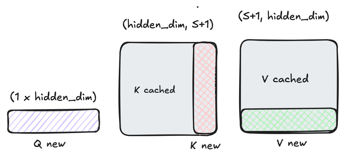
During Token-by-Token Generation (token S+1):
For generating the next token, we only need to compute:
The new attention calculation becomes:
The key efficiency gain comes from:
1. Reusing K^T_cache and V_cache from previous calculations
2. Only computing new key-value projections for the latest token
3. Reducing the attention calculation from O(S^2) to O(S) for each new token
KV caching reduces the total FLOPs by a factor of approximately S for all parts of the forward pass:
In self-attention, we only compute attention for the new token against all previous tokens
In the MLP and LM head components, we only process the new token
The LM head remains the same, but it is such a small fraction of the overall computations that we will skip it in our calculations.
For example, with a 2048-token context:
During pre-fill: ~291 TFLOPs total
For generating token 2049: ~291/2048 ≈ 0.14 TFLOPs
On an H100 GPU (989 TFLOP/s), this would take only:
This is approximately 2048 times faster than the pre-fill phase in terms of pure computation, but remember that we still need to load the entire model parameters (141 GB) from the global memory, and that now we need to also load the KV cache.
KV cache memory footprint can be easily calculated as
For Llama 3.3 70B with 2048 tokens using BF16 precision, this amounts to:
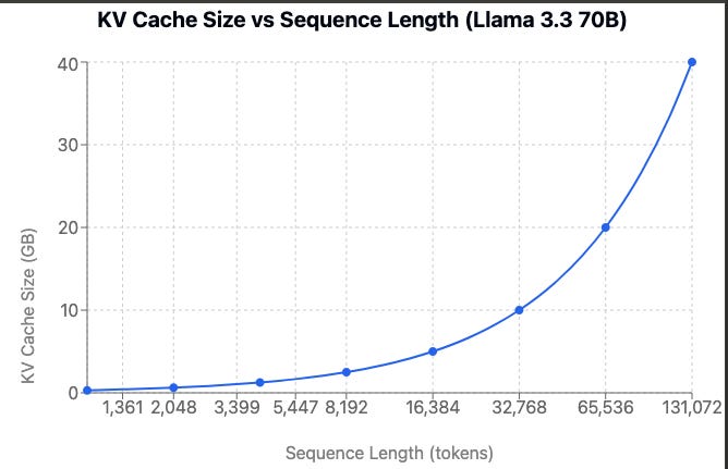
While 671 MB may sound not that significant, this number scales linearly with the batch size (we elaborate on batches later) and with the sequence length (see Fig. 9). This is also the main reason why, at longer sequence lengths, the token-by-token generation* is slower than at shorter sequence lengths-on top of the model weights, the KV cache also needs to be loaded from global memory, increasing processing time for each token produced.
Model weights, plus KV cache, are roughly 141 + 0.6 ≈ 142GB so it takes 142/3350 = 0.04s to load them from the global memory. We calculated above that it only takes 0.00014s to do all computations (assuming 100% compute utilization) - so it takes two orders of magnitude more time to load the model weights than to do the actual computations. This is what we mean by the token-by-token phase of using LLMs being memory bound. We are primarily limited by the time memory transfer takes, not by the speed of compute.
This is one of the insights we hope you take out of reading this article - the token-by-token phase is memory bound; the amount of available compute throughput is of secondary importance, as we massively underutilize the compute resources anyway while waiting for weights to be loaded.
* we use the terms token-by-token phase, decode phase and generation phase interchangeably
Scaling with the input length
One of the main challenges in LLM serving is understanding how input prompt length affects end-to-end performance. Sequence length impacts both the prefill stage and the token-by-token decoding phase, though in fundamentally different ways.
The prompt processing phase exhibits O(N^2) computational complexity; as the sequence length grows, the processing time will grow quadratically*. We derived the FLOPs before as
2 S² hidden_sizefor score matrixQ @ Kᵗ2 S² hidden_sizefor(Q @ Kᵗ) @ V.
This is especially relevant for longer sequence lengths, where the time to the first token will quadratically increase with the length of the input sequence. You can experience this, e.g., when using the long-context Gemini that, as of May 2025, can take up to 2M tokens, but you can wait up to 2 minutes for the first token of the answer to be generated. The intuition you should have developed here is that as the input length keeps increasing, a larger and larger percentage of the total time of processing a request will be spent in prompt processing - the compute-bound part (see Fig. 10).

During the token-by-token phase, the relationship between the generation speed and the sequence length is less straightforward.
FLOP-wise compute is scaling linearly; the new token needs to attend to all of the tokens from the past, or 2 S hidden_size for Q @ Kᵗ and 2 S hidden_size for (Q @ Kᵗ) @ V, but as we already know, FLOPs are not that relevant for the token-by-token case because we are primarily memory bound. What is much more relevant is the size of the data that we need to load from the global memory.
As a reminder, for each forward pass, we need to load the entire model weights from the global memory; on top of this, we also need to load the KV cache from global memory. As we showed in the section above, as we increase the KV cached sequence length, it will occupy linearly more and more memory or by factor S in 2 x bytes_per_param x num_hidden_layers x head_size x num_key_value_heads x S.
Initially the size of the KV cache will be negligible compared to the model size that we need to load, but as we increase the size of the processed prompt, it will occupy an increasingly big portion of the memory (see Fig. 11). Note that if we decide to process larger batches (we discuss this in detail in a later section), the size of the KV cache will grow linearly w.r.t. batch size, as we need to cache the keys and values independently for all examples from the batch. Then at some point the size of the KV cache will overtake the size of the model itself.
The intuition to develop here is that for small batches and short sequences, the sequence length has minimal impact on throughput because loading model weights dominates the memory bandwidth utilization. However, as either batch size or sequence length increases, loading the KV cache takes an amount of time to load for each token, eventually surpassing the time consumed by loading of the model weights themselves.
This transition creates two distinct performance regimes: in the so-called model-dominated regime (short sequences/small batches), throughput remains relatively stable despite increasing sequence length. Once we enter the KV-cache-dominated regime, generation speed begins to degrade in proportion to sequence length. This is largely irrelevant for short sequence lengths but is a significant issue at very long sequence lengths (in the order of tens of thousands of tokens). The additional time loading the KV cache takes scales linearly w.r.t. sequence length.

*In the naive implementations of the attention mechanism memory would also scale quadratically when we realize the SxS score matrix, but flash attention replaces these naive implementations. Flash attention is calculating (Q @ Kᵗ) @ V in an iterative way, where memory required is kept at O(N).
Multi GPU inference
As you might have noted, the 141 GB we need to store the Llama 3.3 70B parameters is more than what we have available on a single Nvidia H100 GPU. H100 cards come with 80GB of HBM memory. We would need a minimum of two to store the model in memory; however, in practice, we would probably like to use more for the KV cache. If we have more memory available, we will be able to allocate a higher proportion of it to the KV cache and a smaller proportion to the model weights, allowing us to run larger batches. We would also linearly increase the available memory bandwidth, at the cost of an increased overhead in cross-GPU communication, though.
Using just two GPUs for Llama 3.3 70B would result in only having a tiny amount of memory available for KV cache because the model weights already take up 88% (141/160=88%) of that memory, leaving only 19GB of memory (160-141=19GB) available for KV cache (in practice even less than that because we can't use 100% of GPU memory but are limited to around 95%). We wouldn’t be able to run large batches nor long sequence lengths; this would be very inefficient. We touch on this in a later section, but being able to run larger batches is the key to enjoying the good inference economics.
GPU servers almost always come in deployments of 4 or 8 GPUs per node, so using 3 GPUs would be wasteful because that would lead to one GPU in the server being entirely unused in a lot of circumstances. Hence, we jump from 2 to 4 GPUs for a single model instance right away.
Let’s assume then we will run the Llama 3.3 70B on 4 H100 cards. There are two main ways to run large-scale AI models on multiple GPUs:
Pipeline parallel
Tensor parallel
Both offer different tradeoffs between throughput and latency. Let’s explore them briefly.
Pipeline parallelism
In the pipeline parallel (PP) setting, we split the model along the layers axis, meaning that each GPU will have a fraction of all layers in the model. E.g., in the case of Llama 3.3 70B with 80 hidden layers served on 4 GPUs, GPU:0 will host the first 20 layers, GPU:1 the next 20, and so on.

The upside of such an approach is the very limited communications between the devices. We only need to broadcast activations from one device to the next one 3 times for a single forward pass.
We can also do pipelining - GPU:0 processes batch 0 and is passing it to GPU:1, then batch 1 is coming in, and GPU:0 can process batch 1 while GPU:1 is processing batch 0, etc. (see Fig. 12). This setting minimizes the stall time of each device, ensuring the maximum throughput; however, it comes at a price - at a single point in time, we only have access to 1/4 of the available compute and memory bandwidth per batch. So generation time is significantly slower than if we were to use all 4 GPUs at the same time.
In practice, orchestrating efficient overlapping batching can be quite challenging; hence, for the remaining part of this text, we will focus on analyzing the far more common tensor parallel setting.
Tensor parallelism
The mainstream parallelism strategy, used by a vast majority of LLM inference providers, is tensor parallelism (TP). In TP, individual neural network layers are split across multiple GPUs, harnessing the combined compute power and memory bandwidth of all devices. This approach significantly shortens per-layer inference time but introduces important trade-offs that must be carefully considered:
Communication Overhead: In regular intervals, e.g., twice per transformer block, the execution must synchronize across GPUs, introducing a significant delay (in the order of milliseconds) per synchronization event. This overhead varies significantly based on interconnect technology (NVLink, PCIe, etc.) and network topology.
Sequential Batch Processing: Unlike pipeline parallelism, TP requires all GPUs to process the same batch simultaneously. A new batch cannot begin until the current one completes, reducing throughput efficiency under dynamic workloads.
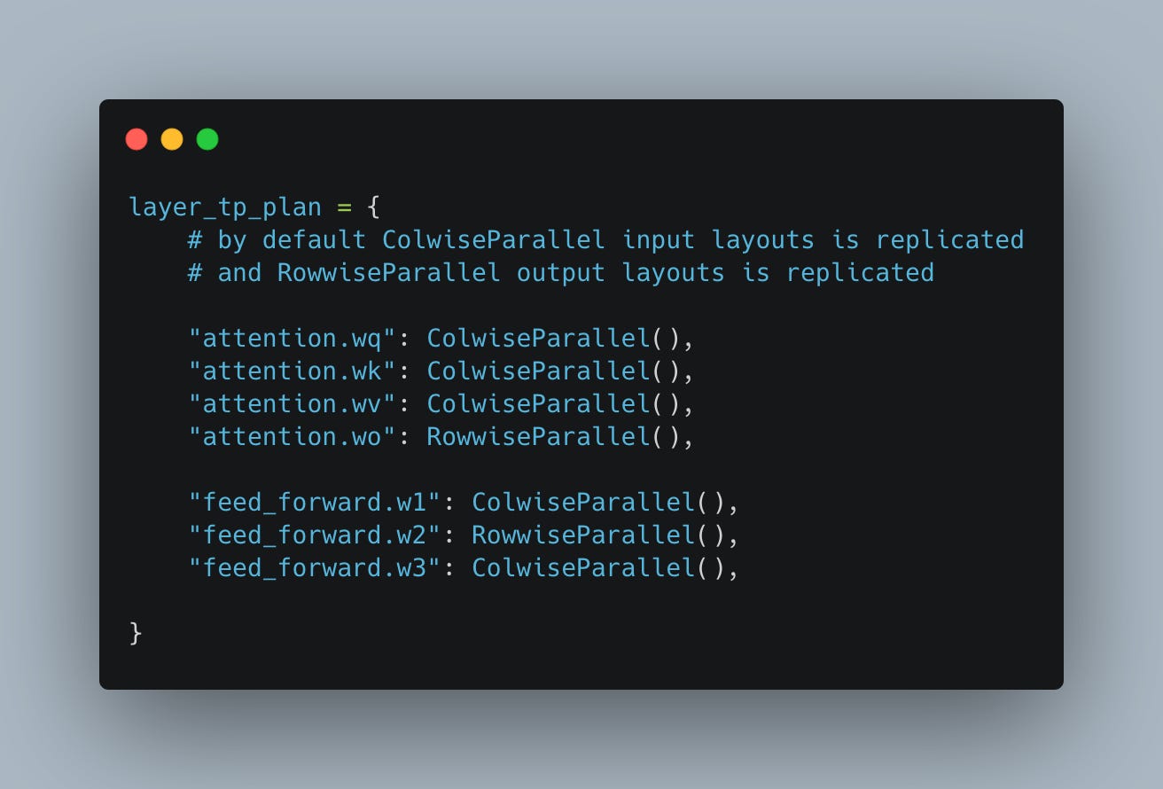
The most efficient parallelization strategy is to have a so-called column-wise split linear layer (we split by the column dimension) followed by the row-wise layer (split across the row dimension). Such a layout minimizes the synchronization to only one sync every two MLP layers.
Mathematical Intuition:
For a weight matrix W₁ split column-wise across 2 GPUs:
Each GPU computes its partial output independently (no communication):
The hidden layer activation becomes:
No communication is needed here because each GPU has all the necessary
data. For the subsequent row-wise split in W₂:
Each GPU computes:
The final output requires an all-reduce sum; in other words, we need to synchronize between the devices:
This layout we can apply to the transformer block, reducing it to only two synchronizations per transformer block (see Fig. 13 and Fig. 14).
Self-Attention: Heads are processed independently, with synchronization only during the output projection (
o_proj).MLP: The up-projection (
w1,w3)is split column-wise and the down-projection (w2)is split row-wise, and the sync is only executed after the down-projection.

Correctly estimating the extra overhead from the coms is quite complicated. In theory, we would need to take into account the two following factors:
Message passing latency: Typically 3-5 μs depending on hardware
Data transfer time: Based on interconnect bandwidth
In an ideal scenario with modern NVLink connections, we could estimate:
The total overhead of 8 or 9 µs would be awesome. However, in practice, it gets much more complicated. During the sync barrier, the compute graph is stalled. We have a constant overhead of a few ms when the GPUs are idling while waiting for the sync to be finished. This extra "tax" is of the main reasons preventing us from utilizing the full memory bandwidth we have available across all the GPUs. Accurately modeling the overhead is quite challenging. As we'll demonstrate in the next sections, the gap between theoretical and actual performance can be quite substantial, requiring empirical measurement for accurate system modeling.
Batching - the key to good economics
As we showed before, during the token-by-token phase, we are primarily memory bound-meaning the main limitation in terms of tokens/s we can get is how fast our GPU is able to load the model weights from the global memory. To generate every single token, we always need to load the entire model.
There is an obvious optimization we could introduce to improve the economics of our operation: run larger batches. Batches are a natural improvement because we can load the model weights once, but we can use the loaded weights to do inference with multiple items from our batch at the same time (and so serve different customers simultaneously).
Increasing the batch size increases the compute usage linearly - we have k times more multiplications to do, but it only marginally changes the memory bandwidth used (only for loading the KV cache), so it's an easy way to increase the compute intensity for our otherwise heavily memory-bound algorithm (to make it less memory-bound). Since the extra memory for the KV cache is significantly smaller than the memory needed for the model, it only adds a small overhead, but it linearly increases the number of produced tokens. We produce twice as many tokens for a batch of 2 and 16x as many tokens with a batch of sixteen.
This is the core message of this post and the main intuition we hope you take away from reading this text: As we grow the batch size, we can effectively share the time to load the model from high bandwidth memory (HBM), aka our cost of loading the model is split across an increasing number of clients, enjoying the economies of scale and decreasing the per-request cost. Having sufficient demand and continuously serving big batches is the key to running a profitable LLM inference business; if you can't support large batches, your cost per token will balloon, making your operation unprofitable.*
*One thing to note is that there is a limit to this model. As we approach really long sequences or really big batches, as we will see in our experiments, the memory footprint of the KV cache starts to slowly overtake the memory footprint of the model itself (see Fig. 15). When this happens, the cost of loading the model will become increasingly irrelevant to the total time of loading data from the global memory.
"Luckily" for us, this situation also has its limit-the memory limit of a GPU node; in the case of H100 cards, it will be 8 × H100 = 8 × 80GB = 640GB. Note how for a batch of 8 at the full context length of Llama, we are already nearly there.

Throughput: theory vs practice
After all of the theoretical introductions, let’s try to combine all that we learned so far to estimate the LLM throughput. We will:
Develop a theoretical performance model based on the GPU spec sheet.
Compare it with a real-world throughput of Llama 3.3 70B on 4 H100 cards.
Explain the discrepancies between theoretical and actual performance.
The time to produce a response to a prompt is a combination of the pre-fill time and the decode time times the number of decode tokens. The more output tokens we produce, the smaller share of time will be spent in the prefill phase. The prefill time is primarily compute-bound, and the time for token-by-token is primarily memory-bound.
Since prefill is so heavily compute-bound, we can estimate the time by dividing the number of floating-point operations during prefill by the total effective FLOPS across all of the GPUs, plus the extra latency from cross-GPU communication time.
The decode time is mainly memory bound, but as we increase the batch size, the compute component will become increasingly important. We will calculate both and take the more significant factor. We also spend some small amount of time in coms.
The simple modeling script is based on what we have discussed above. We take in the model size and its architecture and estimate the throughput we should get given the hardware characteristics.

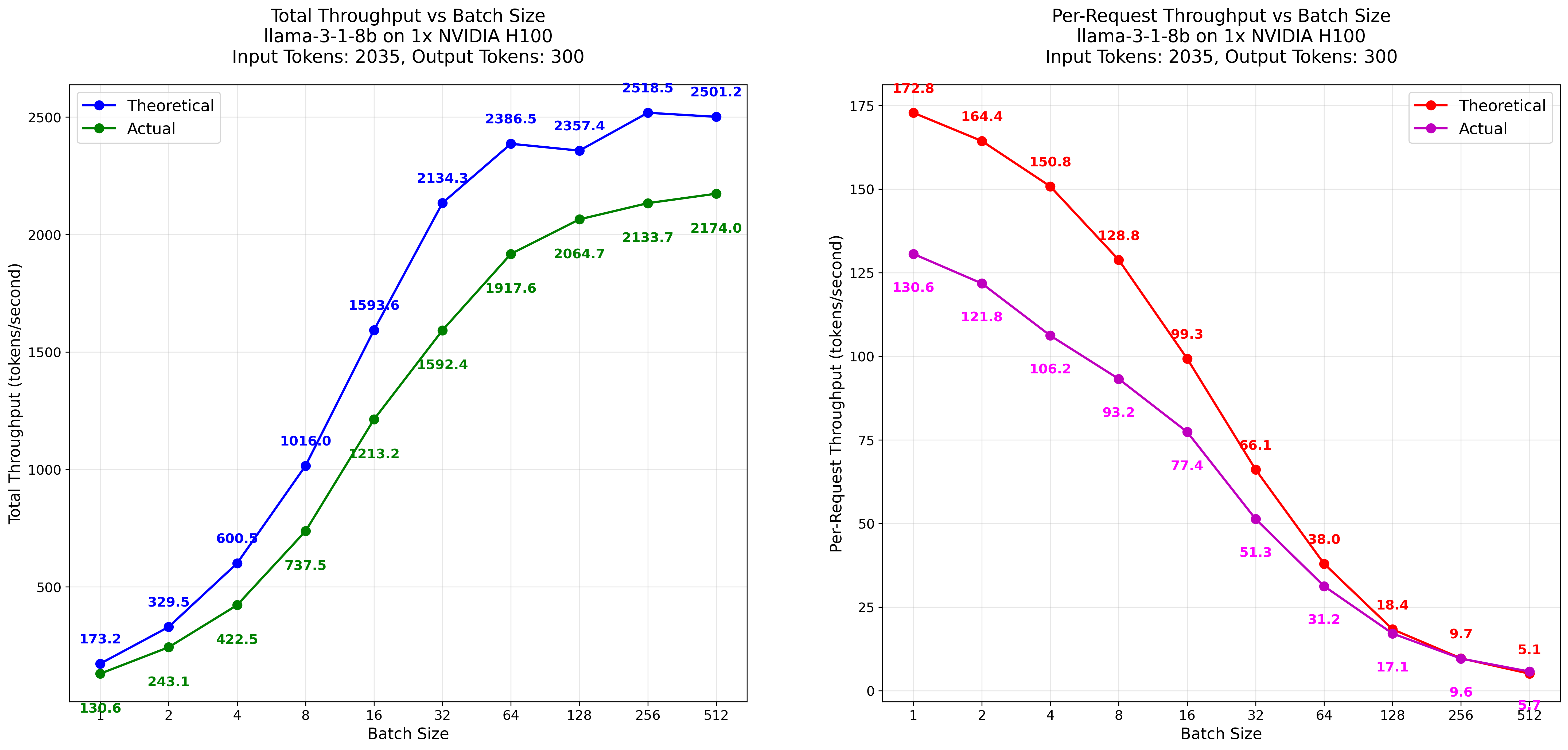
For a Llama 3.3 70B, with 2035 tokens in and 300 tokens out, we will get these estimates:

Let’s first look at the estimated model performance under the different batch sizes. As we derived before, batch size is the single most relevant statistic regarding the tokenomics. Look how the throughput scales nearly linearly with the batch size (see Fig. 16). This is the single most important message you should get out of this text. The key to the good tokenomics is running the models at a large batch size, which is caused by the LLM inference being memory bound, meaning we want to share the cost of loading the model into the memory across as many requests as possible. As the KV cache size is approaching the model size, the total throughput gains are diminishing.
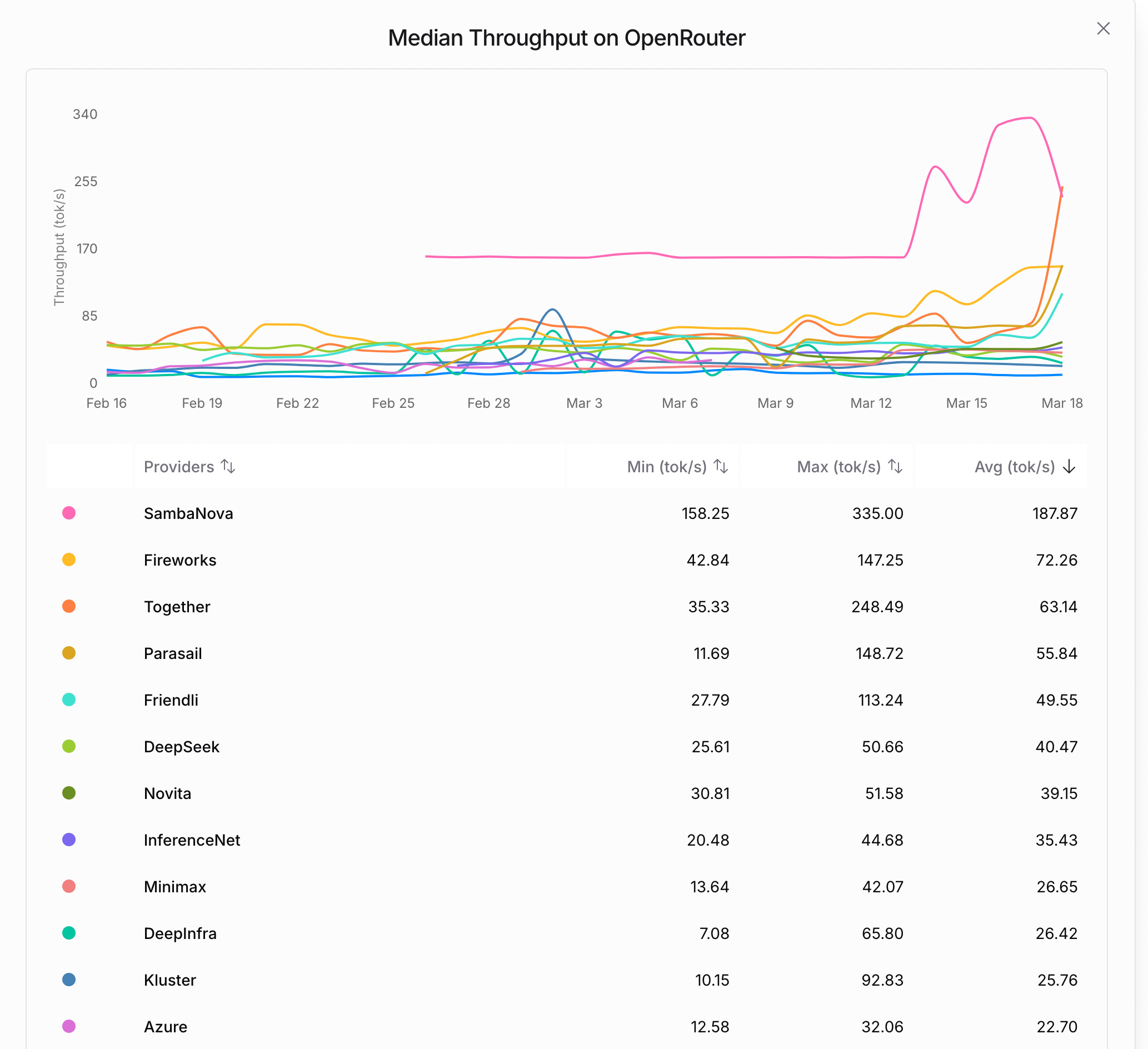
While the total throughput is increasing with the batch size, the per-request speed is decreasing, and the slowdown is accelerating as we increase the batch size due to the increased memory footprint of the KV cache. At some point, with massive batches, the per-request experience will be massively degraded. This means that even if we can support larger batches, e.g., due to the massive demand as DeepSeek experienced in February 2025, we might not want to do so because of the poor token generation speed each user will experience. In general, the variance in speed you experience on OpenRouter (see Fig. 17) can be largely attributed to the current demand, aka the batch size.
It is also part of the reason why the batch API is so much cheaper. In cases where speed is not of utmost importance, an LLM provider can just run massive batches, enjoying economy of scale, with individual requests being handled pretty slowly but processed at a higher profit. There are more nuances to this, e.g., the parallelism strategy (pipeline parallelism offers less cross-device communications overhead), that we consider beyond the scope of this text. We just wanted to give you a real-world example of the real impact of batch size on the price of a generated token.
Now let’s compare the results we get from our model to the actual LLM inference performance. For this, we run a vLLM inference server (a popular LLM serving framework) with Llama 3.3 70B on 4 H100 cards connected with NVLink. The result is quite underwhelming.

max_tokens param to them.
While the general sigmoid-like shape is quite similar, the actual values are very much different. We go from around ~60% of theoretical estimated performance in small batches to around 40%. Where does this difference come from?

Well, this is the problem at the core of GPU optimization - in practice, it is actually extremely hard to properly estimate the wall-time performance of the GPU application. There are many compounding factors here, making the picture more blurry. To mention a few things that are likely contributing to the discrepancy in the observed results vs. reality:
In our model we assumed 100% memory and compute utilization. Theoretical peak performance metrics like TFLOPS and memory bandwidth are never fully achieved in practice. GPUs typically achieve only 50-70% of their theoretical compute capacity due to
Kernel launch overhead and synchronization costs
Memory access patterns that don't perfectly align with cache architectures
Warp divergence and other GPU-specific inefficiencies
Instruction mix that isn't optimal for utilizing all GPU units
… and a lot of other factors
We assumed very little overhead from the cross-device communication; as we explored previously, this is not necessarily the case in practice. In practice, we have tons of other factors that contribute to the potential extra latency, such as
Having to sync the CUDA graph across devices for cross-GPU communication
Synchronization barriers that force all GPUs to wait for the slowest one
internal buffers and management overhead
potential suboptimal (non-coalesced) memory access patterns, especially at larger sizes, with KV caches being stored in random pages of the VRAM memory
and other factors we don’t mention here
For simplicity of calculating FLOPs, we assumed a very naive implementation of the attention mechanism. In practice, everyone is using something like Flash attention. Properly estimating the time and FLOPs involved is quite challenging and complicated and outside the scope of this text.
Overhead coming from the practical implementation of the LLM serving engine, such as paged attention
Extra overhead from using Python, PyTorch, and the vLLM framework itself
We tried to account for some of the above and include them in the extended simulation model. The details can be found in the code, but TL;DR; we assumed decreased compute and memory utilization values, the extra latency from coms, and a few other factors, like extra memory overhead increasing exponentially with the batch size.

While far from perfect, it kind of works. It generalizes pretty well to other sizes; e.g., it works for the Llama 3.1 8B run on TP1.
However, when tried with different batches of different lengths, the differences are more significant, suggesting that the model is far, far from perfect. E.g., we tried estimating the throughput for long context model performance, with 16k tokens in and 1000 tokens out. Due to excessive memory consumption, we kept this setting at a batch size of 8. In such a case, the model failed to correctly predict the final throughput, suggesting that our model is far from perfect.


How challenging it is to correctly predict a model's throughput is another thing that we hope you can take out of reading this text. Accurately estimating it would require a series of very detailed profiling steps, such as profiling the memory access patterns across multiple model sizes, batch sizes, and prompt length combinations; delving deeply into the exact implementation details of (paged) attention implementation; implementation details of the batch scheduling; estimating how different shapes affect the compute and memory utilization; and dozens of different experiments. We deem an accurate estimation across different settings challenging to a degree that it might not be feasible to do so in practice. If you want accurate results, you are probably better off just measuring the real-world results.
From tokens to dollars - estimating tokenomics
As you might know, the pricing of various LLM providers is token-based: you will pay a specific price per million input and output tokens. Some providers use the same price for input and output tokens; others have two distinct prices for input and output tokens.
To summarize what we've learned so far:
The time of prefill is quadratically dependent on the sequence length. As the input size grows, it will occupy an increasingly big percentage of the request processing time.
The time spent generating a single token grows linearly as the context length grows. KV cache will gradually become a more and more substantial percentage of the total data loaded from the global memory (alongside the model parameters).
Since the time of generating a single token can be well approximated by the cost of loading the model weights once from global memory, this time grows linearly with the number of generated tokens.
What should be apparent from the description above is that estimating a fair market price for the input tokens is a non-trivial task. Increased input quadratically increases the cost of prefill, but for standard use cases, prefill is only a minority of the time the GPU spends on processing the request. Then, depending on the batch size and context length and the proportion of these two to the model size, it will affect the throughput.

While estimating a universal proportion of cost between the input and output tokens that generalizes well across all possible shapes of input and output is quite complicated, estimating the cost for a specific input and output config is much simpler. We can just:
Measure the execution wall time.
Assume a fixed ratio
γbetween input and output token costs (e.g.,γ=0.3). There is no deep reasoning behind choosing this particular value ofγwe just need to choose some value.Calculate the per-token cost
βby solving the following equation:
For example, with 2,035 input tokens, 300 output tokens, a batch size of 16, and a runtime of 8.96 second - as we measure in one of the experiments mentioned in the previous section:
Which equals approximately $1.72 per million output tokens and $0.51 per million input tokens.
We apply the same calculations to the different batch sizes based on the experiments we did run in the previous section. As you can see, there is a dramatic price reduction with increasing batch size. The reader should verify that the reduction is directly proportional to the increased total throughput from running larger batches.
Table 1: Estimated cost per 1M tokens for different batch sizes, assuming that the batch is 2035 tokens input and 300 tokens output. The pricing is estimated via the method described in this paragraph.
Obviously, the above is just a single data point from a single experiment for a single pair of input and output tokens. If we change the proportions of input and output tokens, the picture will be very different. To get a more realistic picture, we could, for example, run a Monte Carlo simulation- gathering multiple data points for different input and output configs, calculating the pricing for each example, removing the outliers (e.g., random slower executions due to external factors), and calculating the final price as an average of the median of these samples.
The above strategy still suffers from making very strong assumptions, e.g., we only benchmark the performance of rectangularly shaped inputs-all elements of the batch have the same number of input tokens and the same number of output tokens. We don’t mix the prefill phase with the decode phase-we submit an entire batch at the same time, since all of its elements have the same shape; we expect the prefill to take more or less the same amount of time, after which we only do the decoding part. This is a very strong assumption that is not necessarily going to be the case in the real world. We also hardcoded the value of γ, which is not necessarily fair and optimal for the settings we will be serving.
We’ll pause our pricing model discussion here, and we hope to do a deep dive into more sophisticated pricing strategies in the future text. There are multiple pricing strategies one could use; another interesting angle is estimating the minimal number of users of the LLM model under which an inference is profitable.
Luckily for us, at the end of the day, you can easily verify if you are running a profitable operation. You just add up the profits you made from charging users for input and output tokens, and you verify if this sums up to more than what you paid for renting a GPU for an hour.
Summary
We really hope this text to be a founding block for you to build an accurate world model of LLM inference economics, using Llama 3.3 70B as an example. We start explaining what parameters are present in an LLM, what it means for a model to have 70B parameters, and how the memory is consumed. Then we give you a brief introduction to compute- and memory bandwidth performance and what it means to be compute- or memory-bound, and we explain the concept of FLOP and how many FLOPs are in a matrix multiplication.
We introduce the concept of the prefill phase and the token-by-token phase. We break down FLOPs during different parts of a forward pass, and we show how the prefill is primarily compute-bound. We then explain how different the token-by-token phase is. We introduce the concept of kv-cache; we go again through a forward pass and show how, thanks to the kv-caching, it is now far less dependent on compute (times S less FLOPs), hence how it becomes primarily memory bound. We show how, with the increasing input length, the KV cache occupies an increasingly big portion of the memory load time. We then briefly mention different parallelization strategies, and we describe how extra latency is added when running a multi-GPU setting.
We follow this by introducing the concept of batching. We explain why, since we are primarily memory bound, we can radically improve the economics of our operation by running larger batches. This is the core message of this text and the intuition with which we hope you leave after reading it. We then build a simplified throughput model from first principles and compare its performance to a real-world Llama 3.3 70b run via vLLM. We show the difference between the theoretical performance and a real one, and we give a brief explanation of where the extra overhead is coming from. We show how inaccurate the theoretical model is, which we hope lets you build an intuition about the challenges of predicting real-world performance by a bunch of heuristics.
Lastly, we discuss the challenges of establishing pricing and a fair pricing ratio between input and output tokens. We present a simplified cost model that, while not fully accurate, enables you to build a simple heuristic to price the input and output tokens.
Readers should realize why running on more than the minimal number of GPUs is actually highly beneficial to the inference economics. More GPUs enable higher efficiency through better caching that give a better unit cost per token. With additional GPUs, the same model weights occupy proportionally less of the total memory, allowing more space for KV cache and consequently supporting larger batch sizes. Since throughput scales nearly linearly with batch size, this directly translates to better economics. Each additional GPU also contributes its memory bandwidth to the system, further improving the token generation rate since we are memory-bound in the token-by-token phase.
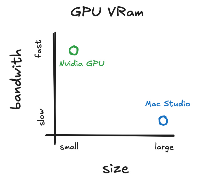
When evaluating hardware for LLM inference, readers should understand that memory size is not the only important factor - memory bandwidth is equally, if not more, critical. Since token-by-token generation is primarily memory-bound, they should always ask, "What is the memory speed?" as this determines how fast models can run. For example, NVIDIA L40S GPUs offer 48GB of memory but with a bandwidth of only 864 GB/s (compared to 3350 in H100 cards), resulting in very slow inference. Similarly, the Apple Mac Studio with M3 Ultra has 512GB of unified memory but only 819GB/s of memory bandwidth (see Fig. 25), limiting its LLM inference capabilities despite the large memory pool.
Readers should also realize why running models on edge devices will always be relatively expensive on a per-token basis. When running on a consumer end device, we are always running batch-size=1. We can’t enjoy the economies of scale from sharing the cost of model load between multiple users. We always bear the entire device and energy cost ourselves. This, combined with the likely suboptimal characteristics of the on-edge hardware and slow memory, will result in high costs such as electricity and hardware depreciation.
The above model is just the tip of the iceberg; we don't discuss any of the possible optimizations, such as speculation models, hardware-specific optimizations, or quantization techniques. The goal of this text is for you to build some basic intuitions on LLM inference. We hope you understand why there are two phases, why one is compute-bound and the other one is memory-bound, and why we hope you developed some intuitions about the relationship between the number of input and output tokens and the request processing time.
To replicate the experiments, find the instructions at Github
@online{tensoreconomics2025llm,
  author = {Piotr Mazurek, Felix Gabriel},
  title = {LLM Inference Economics from First Principles},
  url = {https://www.tensoreconomics.com/p/moe-inference-economics-from-first},
  urldate = {2025-09-17},
  year = {2025},
  month = {May},
  publisher = {Substack}
}
This post alone persuaded me to subscribe, wow. Exactly the sort of quantitatively-flavored explainer I've been looking for.
Wow, can't remember when I read such detailed write up. Are you doing this for work or was hat your Master's degree paper ?
Should I want to build an inference provider business, it would be all in here ! However, too competitive and expensive to launch, but still great insight.
However, I got some real value out of it as I now understand why why I won't get far with my 8GB GPU in my laptop as the KV store for a 131,072 context window would be itself need 40GB (nice diagram !)