DeepSeek Sparse Attention from First Principles

FLOPs, dollars and a path to million-token context window

What sets the DeepSeek team apart among the recent wave of Chinese foundation model labs is the outsized impact of their innovations in model architecture and training. No other team comes close in the breadth of novel techniques the “Whale team” has introduced over the past 24 months. In this text, we conduct a technical deep dive into DeepSeek Sparse Attention (DSA) - the attention mechanism responsible for massively driving down the cost of running the most recent DeepSeek models, especially at long context. This text proceeds as follows:

First, we recall how Group Query Attention works. We show how KV cache scales with the number of tokens in the batch. As we increase the batch size, KV cache quickly becomes the bottleneck, throttling the inference throughput (tokens per second).

Second, we investigate the crucial element of DSA - the Multi-Head Latent Attention (MLA). We explain where the performance gains come from (KV cache compression), we derive a theoretical model, and we compare it with real-world performance on Hopper GPUs with kernels from SGLang.

Last but not least, we cover how DSA itself works. At a high level, DSA reduces the number of tokens each query attends to - similar in spirit to Sliding Window Attention (SWA), but with a crucial difference. SWA attends to a fixed window of the most recent tokens, discarding older context entirely. DSA keeps the full context accessible and uses a lightweight indexer to select the most relevant tokens from anywhere in the sequence. The full MLA attention then runs only over this selected subset. The downside is that we still need to store the full KV cache, but the upside is that empirically it yields far better performance than position-based approaches.

Based on these observations, we speculate about the business implications of DSA - specifically, how it enables “Claude Code-like” products to be viable and profitable at long contexts. We discuss Z.ai’s pricing strategy for the GLM Coding Plan, and mention works building on DSA that could enable even cheaper long-context capabilities.

Introduction

DeepSeek revolutionized the attention mechanism with MLA introduced in DeepSeek V2 back in May 2024. They’ve shown you can compress the keys and values cache into a single compressed representation without sacrificing the performance of the model. The same attention mechanism was later adopted in DeepSeek V3 and R1 that made the DeepSeek team famous. Surprisingly, MLA has been adapted by relatively few competitor models, with notable examples being Kimi K2 adopting MLA and, more recently, GLM 5 adopting DSA.

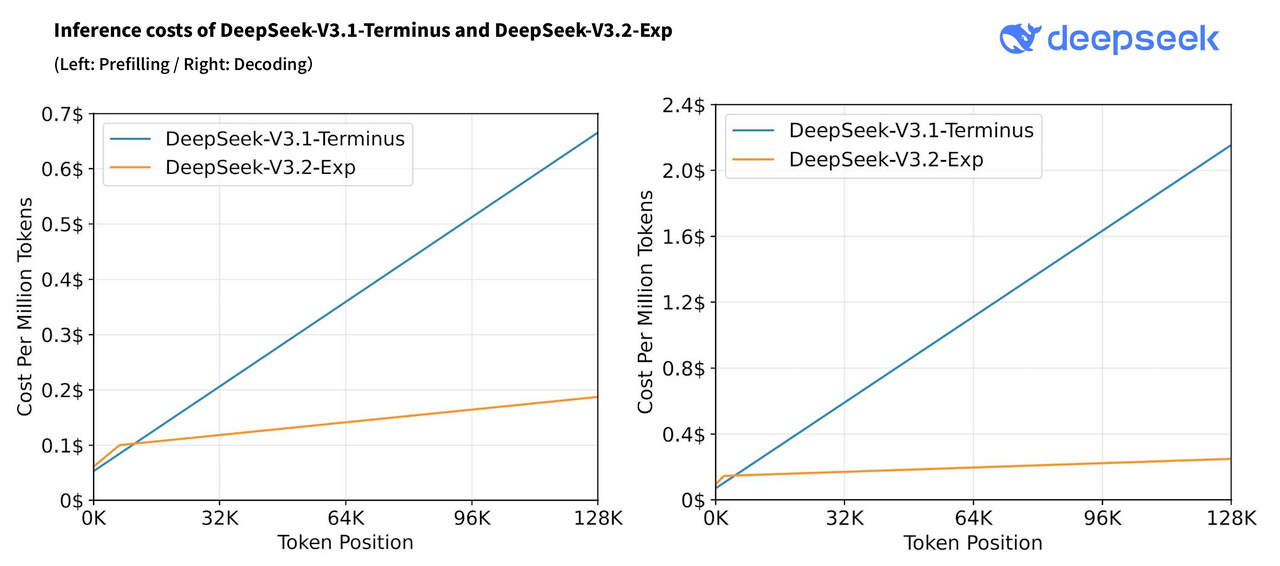
With DeepSeek 3.2, they introduced DeepSeek Sparse Attention (DSA) - optimizing attention further. It achieves near-constant decode time and O(S) prefill, driving down the cost with apparently little to no degradation to performance (e.g., see how well DS 3.2 performs in long-context eval by AA). Figure 1 demonstrates the cost of prefill and decode with sequence length as measured by DeepSeek; later throughout this text we will reference these figures and show how closely we managed to reproduce them.

Figure 1: Estimated cost of prefill and decode for DeepSeek V3.2. DeepSeek.

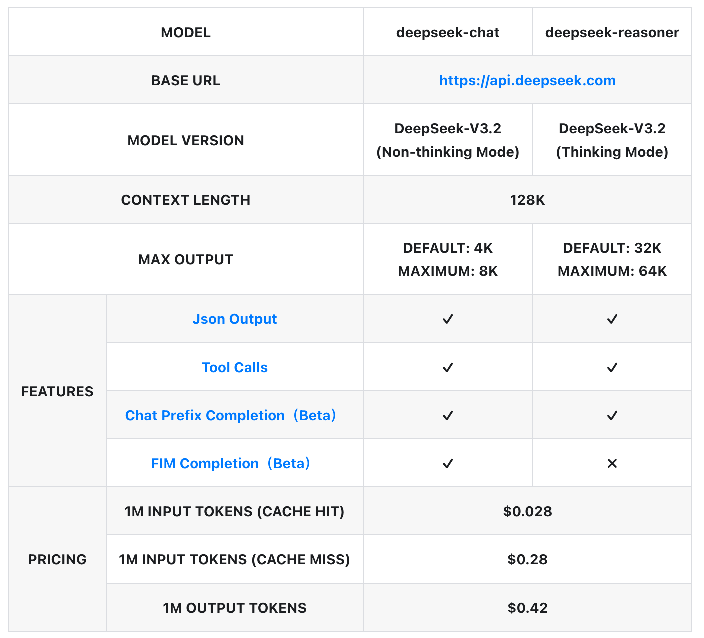
DSA enabled DeepSeek to drive down the price of the API to only 42 cents per million output tokens, fueling the intelligence involution race (see Fig. 2 demonstrating DS pricing).

Figure 2: DeepSeek 3.2 official pricing as of 12.04.2026. https://api-docs.deepseek.com/quick_start/pricing

To fully enjoy this article, the reader needs some prior knowledge: what it means to be compute/memory bound, what a FLOP is, the difference between prefill and decode, etc. If these topics are new, we recommend reading the seminal tensoreconomics text first:

LLM Inference Economics from First Principles

Group Query Attention

Before we introduce MLA, let’s take a look at “vanilla” multi-head attention. At the core of it is the attention equation. This computation is executed independently for each attention head.

\(\text{Attention}(Q, K, V) = \text{softmax}\left(\frac{QK^T}{\sqrt{\text{head_dim}}}\right)V \tag{1}\)

Where:

\(S \text{ is the sequence length}\)

\(\mathbf{Q} \in \mathbb{R}^{S \times \text{head_dim}}\)

\(\mathbf{K} \in \mathbb{R}^{S \times \text{head_dim}}\)

\(\mathbf{QK}^T \in \mathbb{R}^{ S \times S}\)

\(\mathbf{V} \in \mathbb{R}^{S \times \text{head_dim}}\)

\(\mathbf{QK}^T\mathbf{V} \in \mathbb{R}^{S \times \text{head_dim}}\)

After we calculate this for each attention head, we concatenate across the head_dim dimension and multiply the result by the Wo projection matrix.

\(\mathbf{W}_O \in \mathbb{R}^{\text{hidden_size} \times \text{hidden_size}}\)

\(\text{MultiHead}(Q, K, V) = \text{Concat}(\text{head}_1, ..., \text{head}_h)W_O\)

\(\mathbf{O}_{\text{proj}} \in \mathbb{R}^{S \times \text{hidden_size}}\)

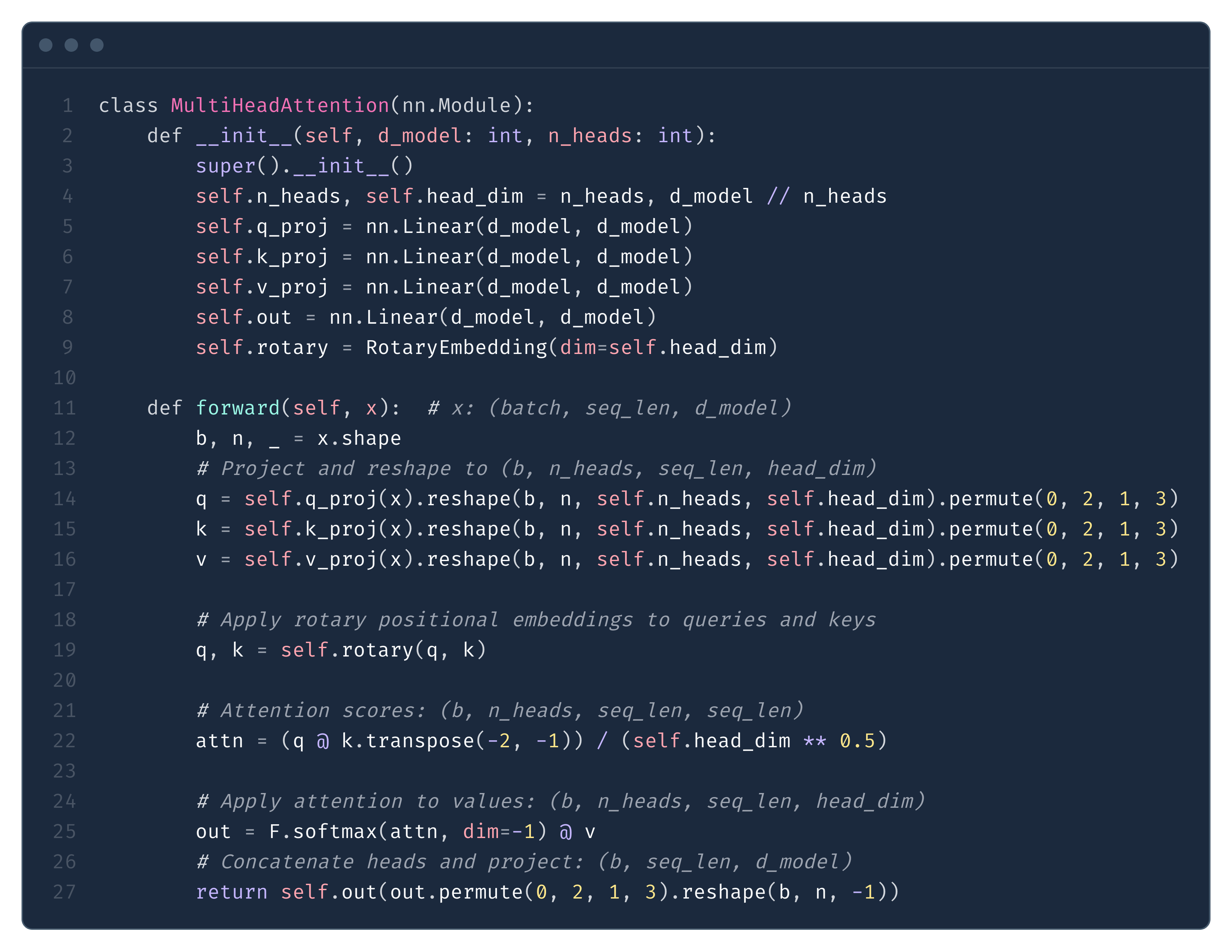
The prefill computation couldn’t be more straightforward. We present an example forward pass of MHA in Figure 3.

Figure 3: Multi-head attention prefill forward pass.

As we have shown in the formative article of tensoreconomics, prefill is primarily compute-bound, meaning we spend most time actually running the computations (we do large-scale matrix multiplications) - hence the FLOPs will determine the runtime. We can estimate the self-attention prefill FLOPs as:

Since all attention is causal, each token attends only to itself and prior tokens — the exact count is S(S+1)/2 pairs, which we approximate as S²/2 for large S. The W_o projection is applied to every token unconditionally, so it is unaffected.

\(\text{FLOPs}_{QK^T} \approx 2 \cdot \text{num_attention_heads} \cdot \frac{S^2}{2} \cdot \text{head_dim} = S^2 \cdot \text{hidden_size}\)

\(\text{FLOPs}_{(QK^T)V} \approx 2 \cdot \text{num_attention_heads} \cdot \frac{S^2}{2} \cdot \text{head_dim} = S^2 \cdot \text{hidden_size}\)

\(\text{FLOPs}_{W_O} = 2 \cdot S \cdot \text{hidden_size} \cdot \text{hidden_size} = 2 \cdot S \cdot \text{hidden_size}^2\)

\(\text{FLOPs}_{\text{total}} = 2 \cdot S^2 \cdot \text{hidden_size} + 2 \cdot S \cdot \text{hidden_size}^2 \tag{2}\)

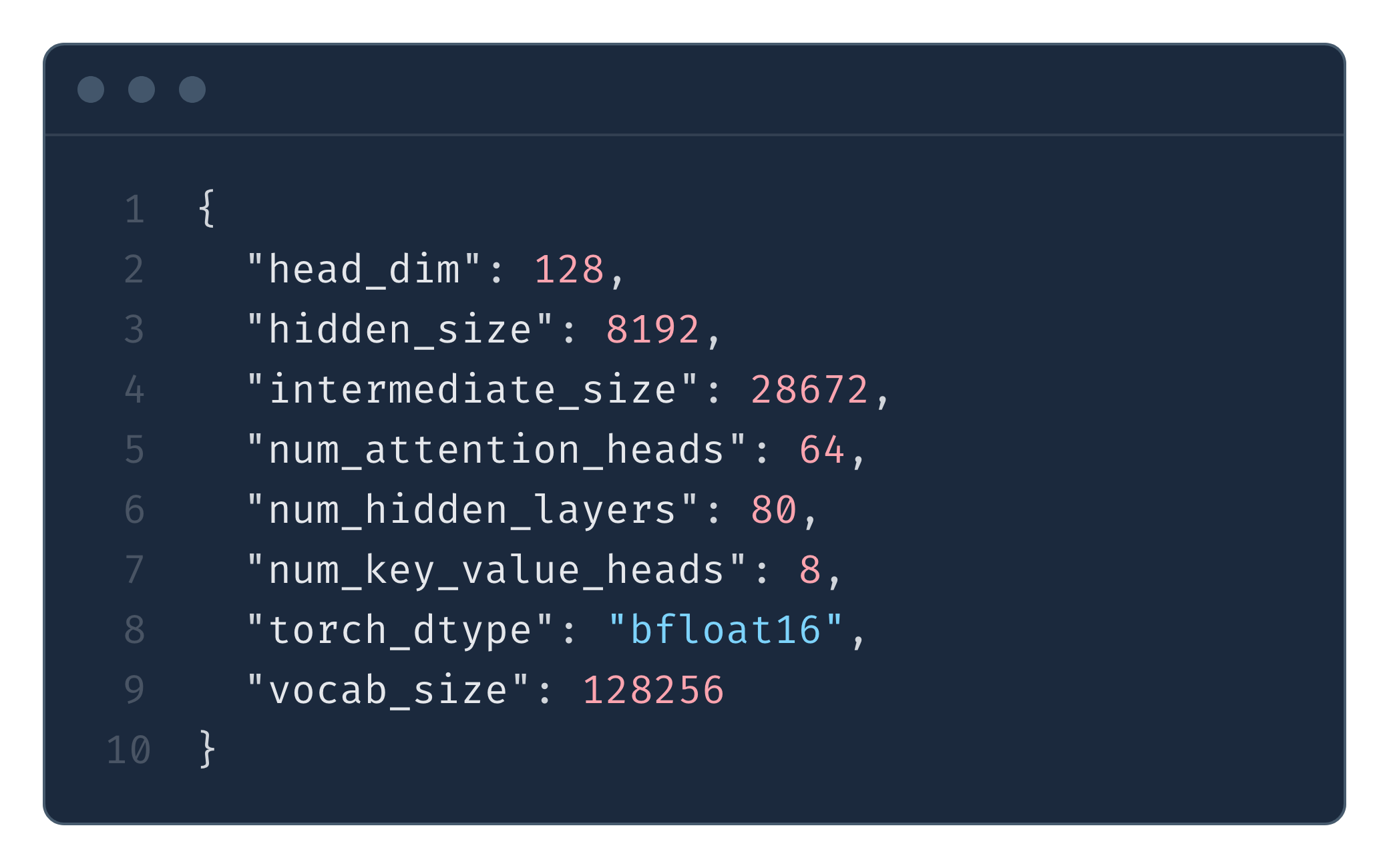
To make our calculations in this section more concrete, we will be using Llama 3.3 as an example. For parameter names, we follow the Hugging Face config. For further details see Fig. 4.

Figure 4: Config of Llama 3.3 that we will be using throughout the next few paragraphs as a reference model.

In Fig. 5 we present the results of an experiment showing how the latency of an attention layer forward pass increases as we scale batch size and the sequence length. Notice how the time (because of the underlying FLOPs increase) of the forward scales quadratically with sequence length but linearly with the batch size. It is consistent with Eq. (2), where we can see that the FLOPs scale with S², and since prefill is compute-bound, so should the latency.

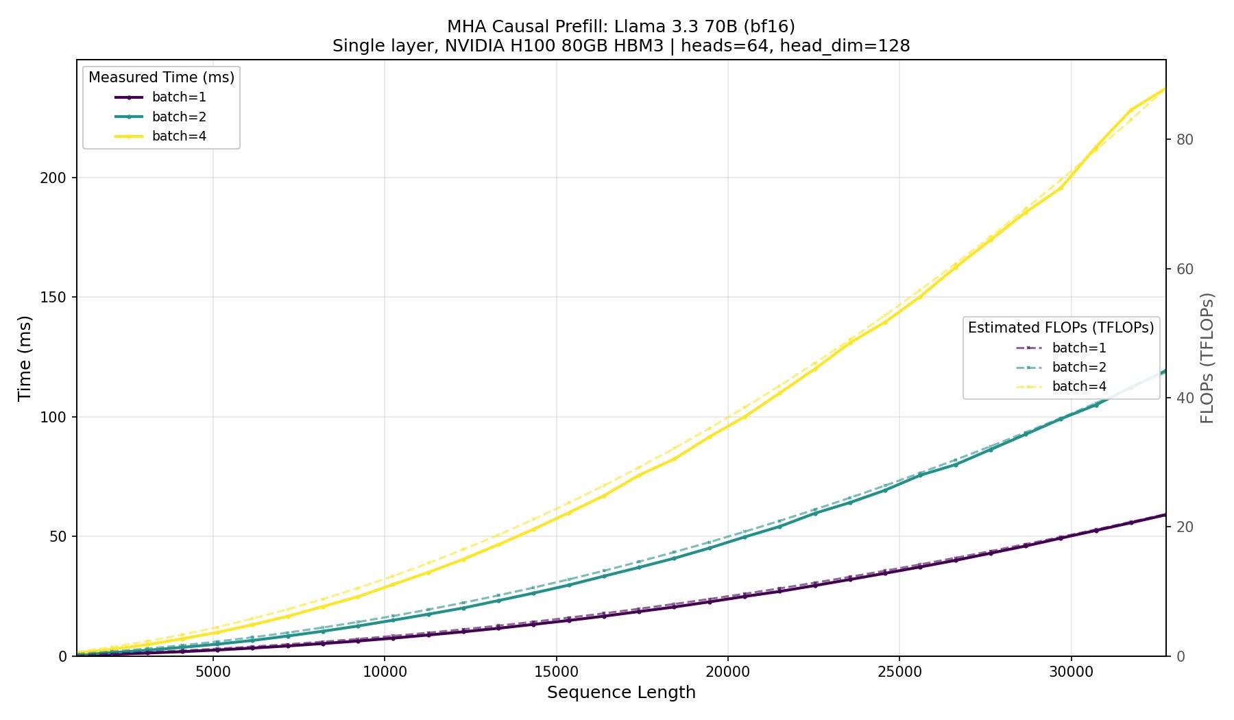
Figure 5: MHA causal prefill benchmark on H100 (single layer, 64 heads, head_dim=128, 32 sequence lengths from 1K to 32K, batch sizes 1/2/4). Solid lines show measured wall-clock time; dashed lines show estimated FLOPs using Eq. (2). Benchmark uses PyTorch’s scaled_dot_product_attention.

Note how GPU compute (FLOPS) is a good predictor of latency. H100 offers ~989 TFLOPS, and we can estimate the latency as:

\(\text{latency} \approx \frac{\text{FLOPs}}{\text{GPU peak FLOPS}} \times \text{model flop utilization (MFU)} \tag{3}\)

For an attention operation, we get a consistent ~43% MFU across different batch sizes and sequence lengths. For example, at batch=4 and S=8192, the causal attention totals 8.8 TFLOPs.

\(\text{latency} \approx \frac{8.8 \text{ TFLOPs}}{989 \text{ TFLOPS}} \times \frac{1}{0.43} = 8.9 \text{ ms} \times 2.33 = 20.7 \text{ ms}\)

basically the exact time we observe in Figure 5.

This quadratic scaling of prefill will be in stark contrast with decode - in decode, the time of a single forward pass scales linearly with the sequence length. Since in a typical GPU workload decode dominates the wall time, and hence determines the end-to-end inference cost, in this text we will mostly focus on decode.

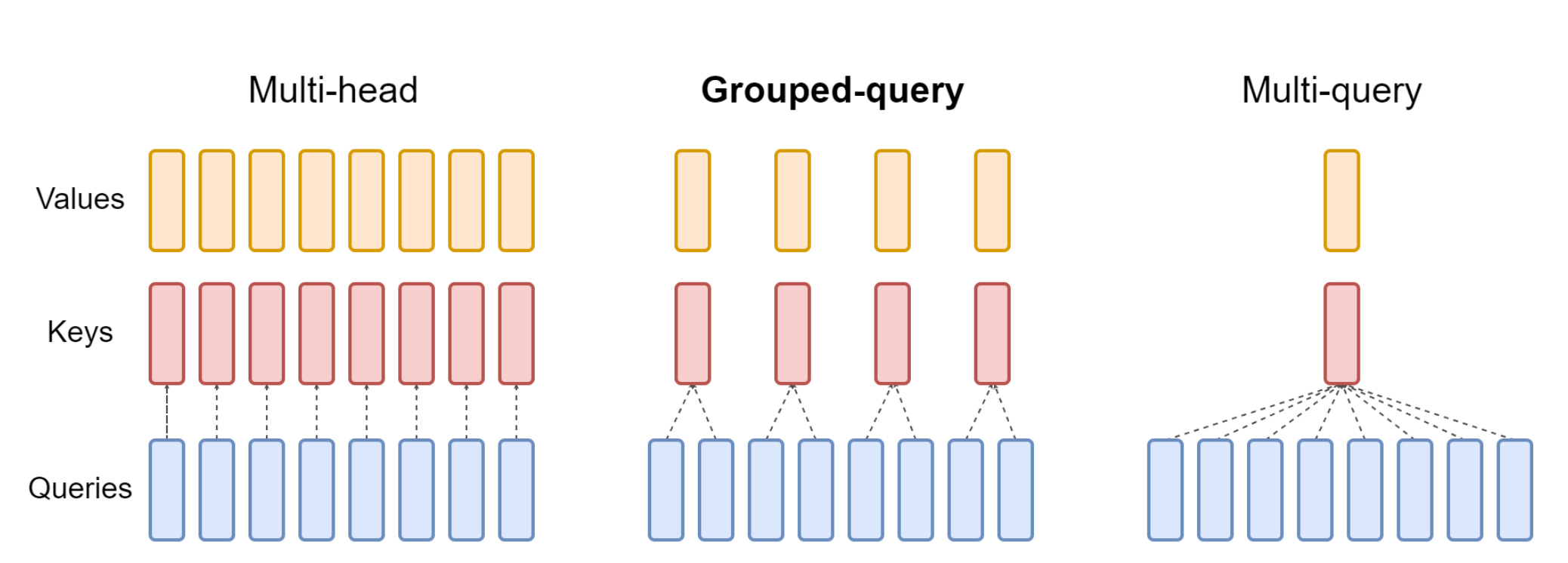
Before we proceed to the decode phase, we need to introduce the concept of Group Query Attention (GQA). GQA was introduced back in 2023 by a team at Google and is considered the de facto standard today for attention-based models. All models you might know, like Llama, Qwen3, gpt-oss and others, use this technique.

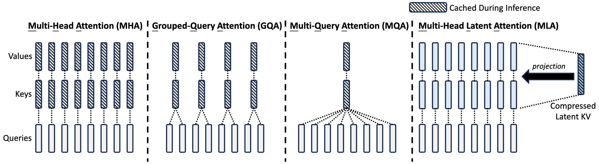
The concept is pretty well captured by the visualisation we present in Fig. 6. GQA reuses single key and value projections across multiple attention heads. As we will show in the next section, it has an enormous impact on the inference speed and, as a result, the cost of producing a token. For this reason, GQA has been largely adopted in the industry and is powering a significant portion of the leading open-source models.

Figure 6: “Overview of grouped-query method. Multi-head attention has H query, key, and value heads. Multi-query attention shares single key and value heads across all query heads. Grouped-query attention instead shares single key and value heads for each group of query heads, interpolating between multi-head and multi query attention.” GQA paper.

However, there are no free lunches. Using GQA attention comes at a cost of worse end-to-end model performance, as demonstrated in Tab. 1. Even after adjusting for an equal number of parameters, the DeepSeek team showed that using GQA results in a slightly worse performance.

Table 1 | Comparison among 7B dense models with MHA, GQA, and MQA, respectively. MHA demonstrates significant advantages over GQA and MQA on hard benchmarks. ... All of these three models are trained on 1.33T tokens, and share the same architecture except for the attention mechanisms. In addition, for a fair comparison, we align the number of parameters of them to around 7B by adjusting the number of layers. DeepSeek V2.

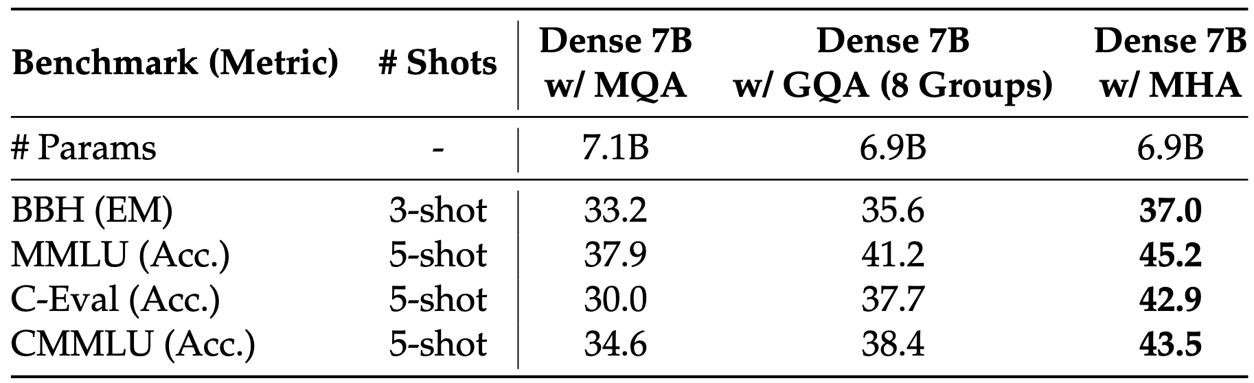
This begs the question: why do people design models with GQA? Why is reducing the number of keys and values cached relevant for reducing the cost of inference?

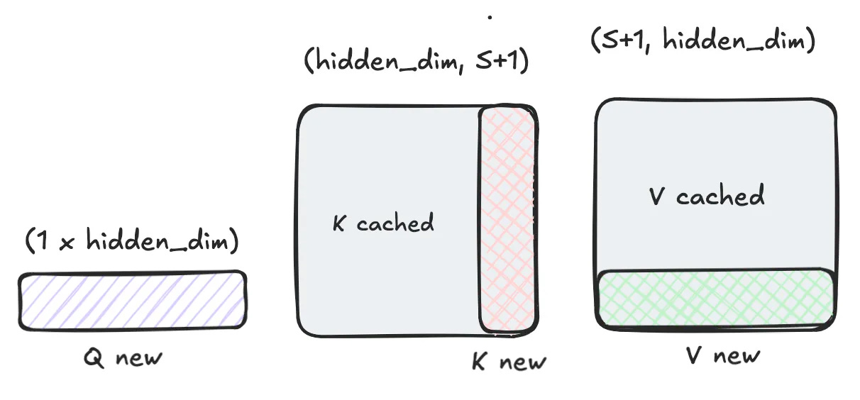
During the decode, we can cache the keys and values for past tokens and calculate the output only for the new token. The math works similarly to prefill, with an adjustment that now “sequence length” is just 1 (for batch size 1):

\(S \text{ is the cached sequence length (all previous tokens)}\)

\(\mathbf{Q} \in \mathbb{R}^{1 \times \text{head_dim}}\)

\(\mathbf{K} \in \mathbb{R}^{(S+1) \times \text{head_dim}}\)

\(\mathbf{QK}^T \in \mathbb{R}^{1 \times (S+1)}\)

\(\mathbf{V} \in \mathbb{R}^{(S+1) \times \text{head_dim}}\)

\(\mathbf{QK}^T\mathbf{V} \in \mathbb{R}^{1 \times \text{head_dim}}\)

We repeat this for each head independently. As you can see visualised in Fig. 7, for this to work we need to save (cache) the k and v values for the past tokens. This scales linearly with the number of tokens in sequence (S).

Figure 7: KV cache concept visualised. We need only to calculate the query, key, and a value for the new token.

The memory we need to allocate for caching scales as follows:

\(\begin{aligned} \text{KV Cache Size per token in MHA} = \; & 2 \cdot \text{num_attention_heads} \cdot \text{head_dim} \\ & \cdot \text{precision} \cdot \text{num_layers} \end{aligned} \tag{4}\)

E.g., for Llama 3.3 70B stored in bf16, this would amount to:

\(\begin{aligned} \text{KV Cache Size per token} &= 2 \; (\text{K and V}) \cdot 64 \; (\text{heads}) \cdot 128 \; (\text{head_dim}) \\ &\quad \cdot 2 \; (\text{bytes}) \cdot 80 \; (\text{layers}) \\ &= 2{,}621{,}440 \text{ bytes} \approx 2.6 \text{ MB} \end{aligned}\)

for each token in the sequence (S).

The innovation of GQA is that we reuse a single KV projection between multiple heads. In the HF config (see Fig. 4), this is stored under the num_key_value_heads. Typically there will be far fewer key value heads than the attention heads; e.g., in Llama 3.3 70B, it is 8 key value heads vs 64 attention heads. This means that the memory footprint per token is reduced 8x, which has a significant impact on the inference speed.

\(\begin{aligned} \text{KV Cache Size per token in GQA} = \; & 2 \cdot \text{num_key_value_heads} \cdot \text{head_dim} \\ & \cdot \text{precision} \cdot \text{num_layers} \end{aligned} \tag{5}\)

As expected, it reduces the size we need to keep per token 8 times:

\(\begin{aligned} \text{KV Cache Size per token} &= 2 \; (\text{K and V}) \cdot 8 \; (\text{KV heads}) \cdot 128 \; (\text{head_dim}) \\ &\quad \cdot 2 \; (\text{bytes}) \cdot 80 \; (\text{layers}) \\ &= 327{,}680 \text{ bytes} \approx 328 \text{ KB} \end{aligned}\)

In Fig. 8 we present a simple implementation of GQA in decode mode. The implementation is very similar to MHA, with the key difference being repeat_interleave, where we repeat the tensors so they can be re-used by multiple attention heads.

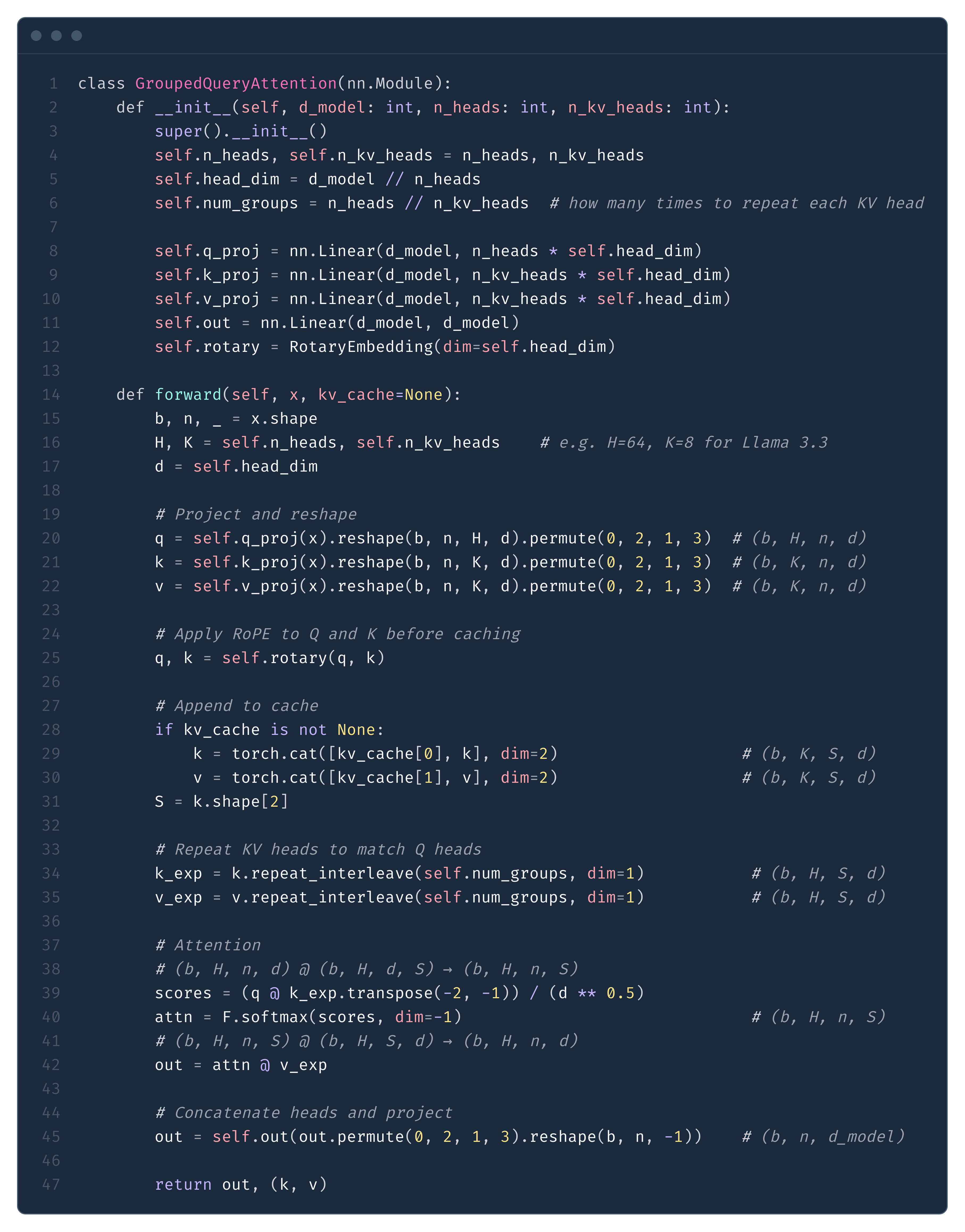
Figure 8: GQA decode forward pass. Queries project to all H heads while keys and values project to K < H heads, then are repeated via repeat_interleave to match. The KV cache stores separate K and V tensors of size n_kv_heads x head_dim each.

Because of KV caching, during decode we move from the matrix-matrix multiplication regime into matrix-vector multiplication. This has an enormous impact on the FLOPs - compare Eq. (6) below with the prefill FLOPs in Eq. (2): the S² term becomes S, scaling down by a factor of S.

\(\text{FLOPs}_{QK^T} = 2 \cdot \text{num attention heads} \cdot 1 \cdot S \cdot \text{head dim} = 2 \cdot S \cdot \text{hidden size}\)

\(\text{FLOPs}_{(QK^T)V} = 2 \cdot \text{num attention heads} \cdot 1 \cdot S \cdot \text{head dim} = 2 \cdot S \cdot \text{hidden size}\)

\(\text{FLOPs}_{W_O} = 2 \cdot 1 \cdot \text{hidden size} \cdot \text{hidden size} = 2 \cdot \text{hidden size}^2\)

\(\text{FLOPs}_{\text{total}} = 4 \cdot S \cdot \text{hidden size} + 2 \cdot \text{hidden size}^2 \tag{6}\)

This should make intuitive sense - for each new token we need to calculate attention to all previous tokens - O(S) scaling with respect to sequence length. However, as the seasoned readers of our publication will know, now we hit another problem - we get into the low arithmetic intensity regime, and the speed of our program is now limited by the speed of GPU memory, or, in other words, we become memory-bound.

The bottleneck is no longer how fast the GPU can compute but how fast it can load data from HBM (high-bandwidth memory) into the compute units - and this is why the size of the KV cache matters so much for decode performance.

For each transformer layer we have to:

• Load the Wq, Wk, Wv and Wo projection matrices.

• Load the MLP layer (or multiple experts in MoE models).

• Load the past KV cache.

All this memory loading will take time, and this time will ultimately determine our cost of serving the model. The issue is, as we increase the combined sequence length, either through processing a longer sequence for one user or via combining multiple requests from multiple users into a single batch request, the size of the KV cache will increase linearly with the number of tokens cached.

The reader should note that, while the size of the KV cache will scale linearly with the batch size, the memory footprint of attention and MLP weights remains constant - we load them once and reuse them across all requests in the batch.

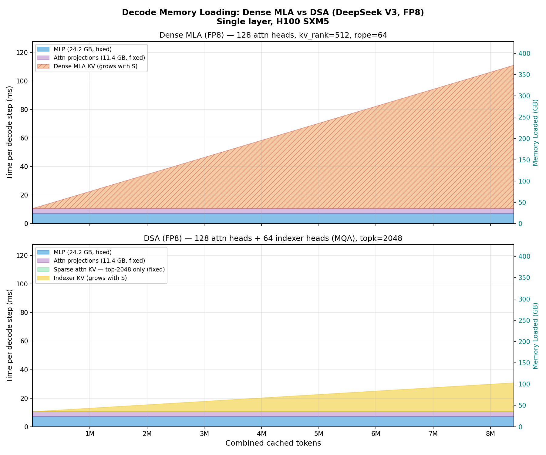
To better illustrate this point, please look at Figure 9. As we increase the combined cached sequence length, at some point the KV cache starts to dominate the memory footprint. Note that this is the memory that GPU(s) needs to load each time we do a forward pass.

Figure 9: Estimated memory loaded per decode step for different numbers of cached tokens. This is a calculation using the config of Llama 3.3 70B, assuming 2 bytes per parameter and storing KV cache in bf16. Note that this is not the total memory footprint a model needs to load; we also need to load embeddings, the LM head and some values for RMS norm. We skip them for the sake of simplicity. For calculating the memory footprint of different models, we recommend the LM cache calculator: https://lmcache.ai/kv_cache_calculator.html

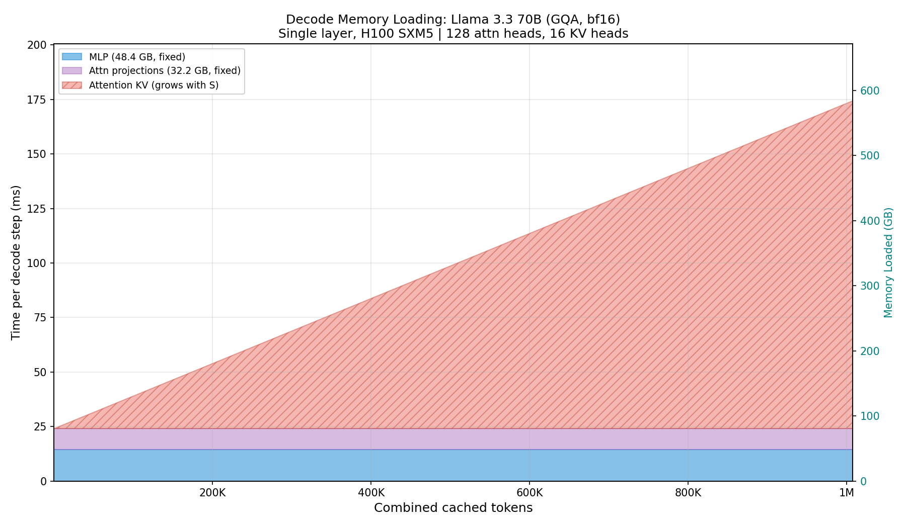
The KV cache growing linearly with the batch size (we store KV for each sequence independently) is the ultimate reason why, as we increase the batch size, the time of a forward pass increases, throttling throughput measured in tokens per second (tps).

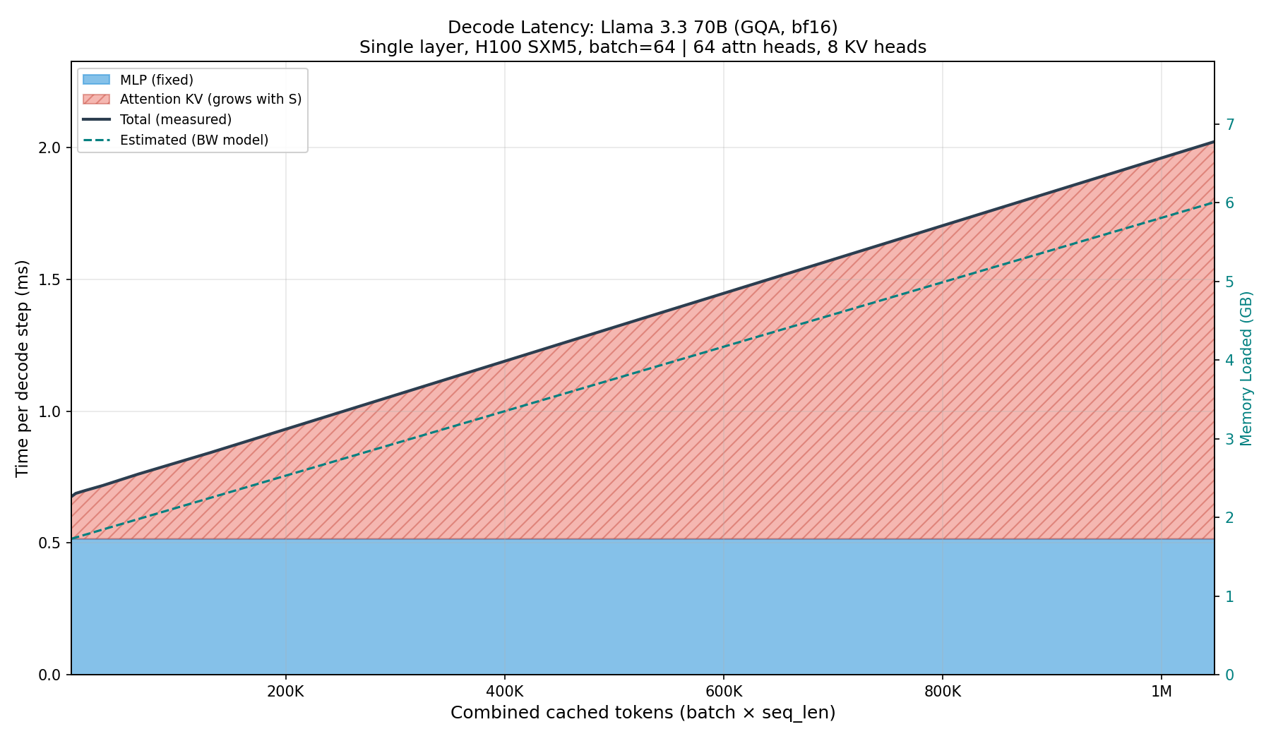
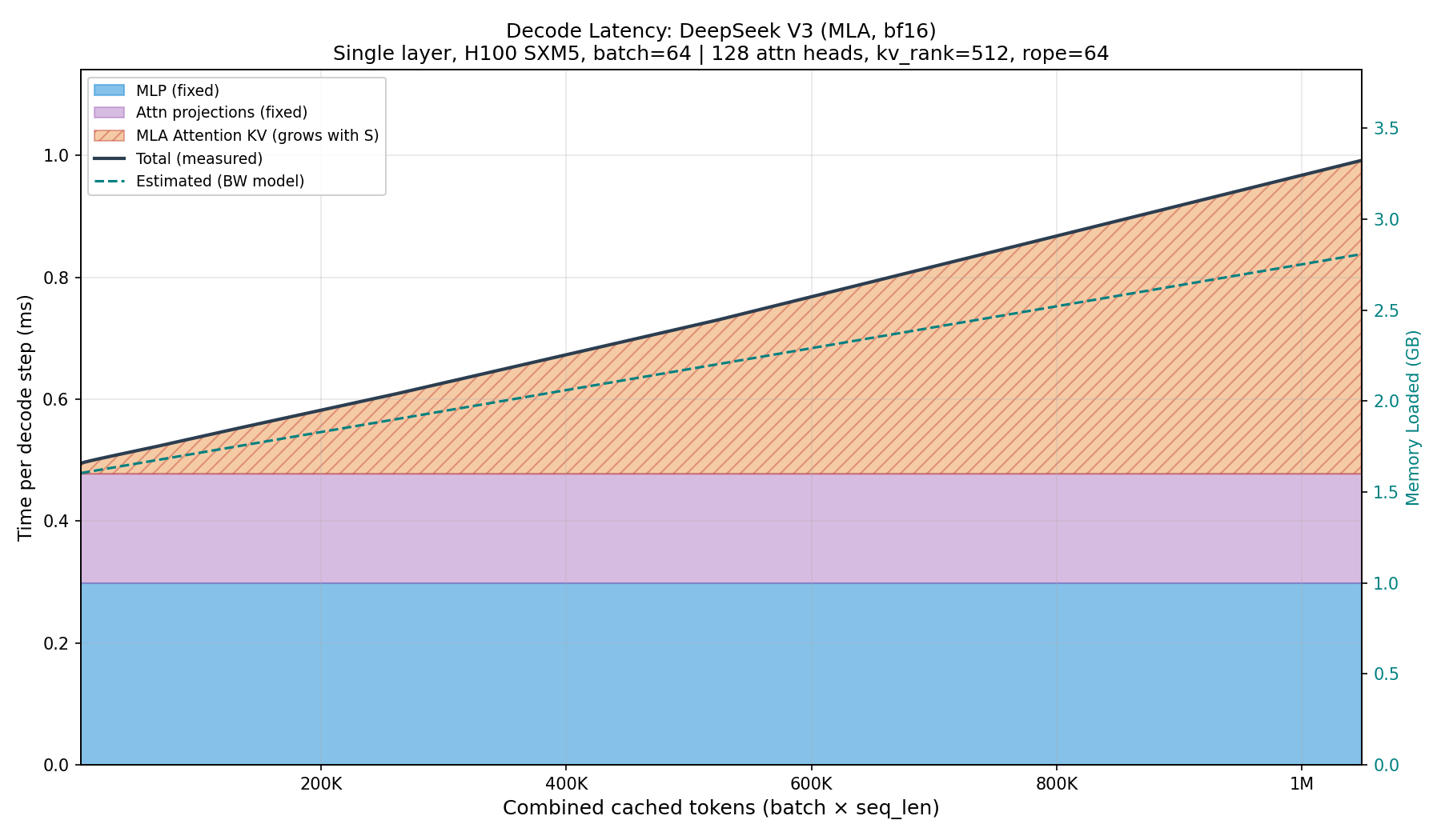
This is not just a theoretical argument. In Figure 10 we fix the batch size at 64 and scale the sequence length, measuring the wall time of each component. Note how the measured latency closely follows the shape predicted by the memory loading model in Fig. 9.

The computation in Fig. 10 is for a single layer due to compute constraints (to decrease the complexity, we limited the experiments to a single H100 instance), but the exact same pattern will emerge when we run the actual Llama inference; it will be just repeated by the number of transformer layers.

Figure 10: Measured GQA decode latency for one transformer layer on H100 SXM5, batch=64, Llama 3.3 70B config (bf16). MLP (blue) is fixed regardless of sequence length. Attention KV (red, hatched) grows linearly as more cached tokens must be read from HBM. The teal dashed line shows the time predicted by dividing total memory loaded by H100 HBM bandwidth (3.35 TB/s) - the close match confirms decode is memory-bandwidth bound. Compare with the theoretical prediction in Fig. 9. Benchmark uses flash attention.

The main intuition the reader should take from reading this section is that for cloud-based inference, where we operate at large batches, the KV cache is becoming the bottleneck throttling the end-to-end throughput (tps). Even though GQA reduces the memory footprint of KV cache, it remains a significant factor limiting the inference speed. The intuitive solution to this problem is to try to compress the size of the KV cache even more, and this is the exact motivation behind Multi-Head Latent Attention.

Multi Head Latent Attention (MLA)

MLA was introduced in May 2024 in DeepSeek V2. The core idea is pretty well captured by Fig. 11 - instead of caching keys and values, why not cache a single compressed (latent) representation for both of them and then simply train two projection matrices to project from latent representation into keys and values? This way we need to store and load during inference significantly less data, speeding up the decode.

Figure 11: “Simplified illustration of Multi-Head Attention (MHA), Grouped-Query Attention (GQA), Multi-Query Attention (MQA), and Multi-head Latent Attention (MLA). Through jointly compressing the keys and values into a latent vector, MLA significantly reduces the KV cache during inference.” DeepseekV2 paper.

In the DeepSeek ablation studies, they show that MLA leads to better end-to-end results than MHA (Tab. 2), while requiring significantly less memory to cache during decode. This is in contrast to GQA, which reduces memory but degrades quality (Tab. 1). According to the DeepSeek V2 paper, this was the main motivation - compress the KV cache to make inference cheaper without compromising model quality.

Table 2 “Comparison between MLA and MHA on hard benchmarks. DeepSeek-V2 shows better performance than MHA, but requires a significantly smaller amount of KV cache ... For a solid conclusion, we train and evaluate models across two scales. Two small MoE models comprise about 16B total parameters, and we train them on 1.33T tokens. Two large MoE models comprise about 250B total parameters, and we train them on 420B tokens. Also, two small MoE models and two large MoE models respectively share the same architecture except for the attention mechanisms.” DeepSeekV2 paper.

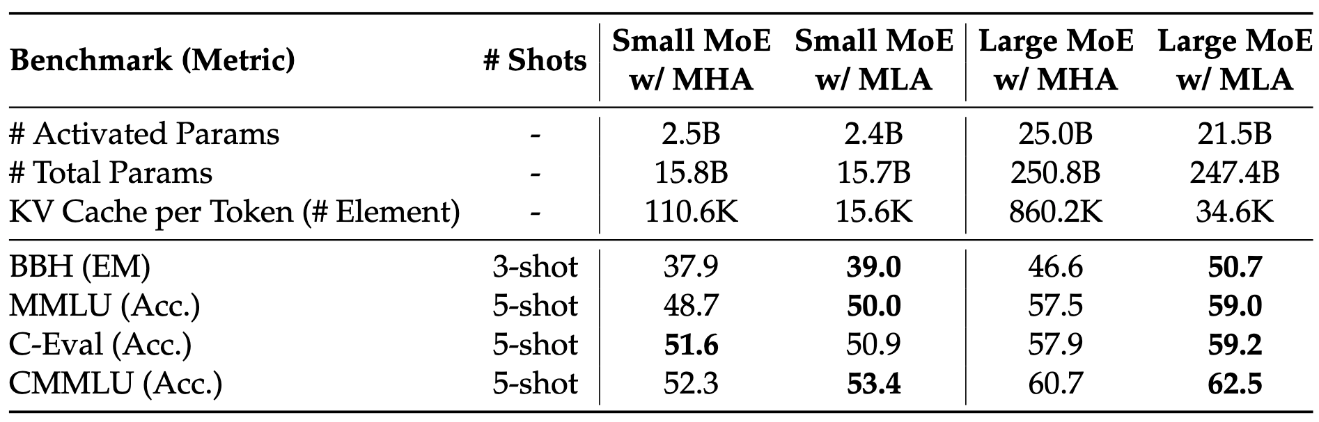
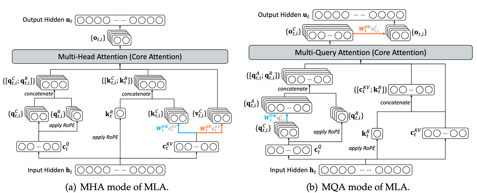
MLA can be executed in two mathematically equivalent modes (Fig. 12): MHA mode and MQA mode. In MHA mode, we reconstruct the full keys and values from the compressed latent and run standard multi-head attention. This minimizes FLOPs, which is what we want during prefill, where we are compute-bound. In MQA mode, we instead absorb the key projection into the query and attend directly to the compressed latent. This spends extra FLOPs, but during decode we are memory-bound anyway, and in return we significantly reduce the memory loaded per step because we only need to pull in the single compressed latent instead of per-head K/V. In the following walkthrough we derive the math for MQA mode that enables fast decode; we discuss why MHA mode is better for prefill in the Appendix.

Figure 12: Illustration of the MHA and MQA modes of MLA. For DeepSeek-V3.1-Terminus, the MHA mode is used for training and prefill, while the MQA mode is used for decode. DeepSeek 3.2.

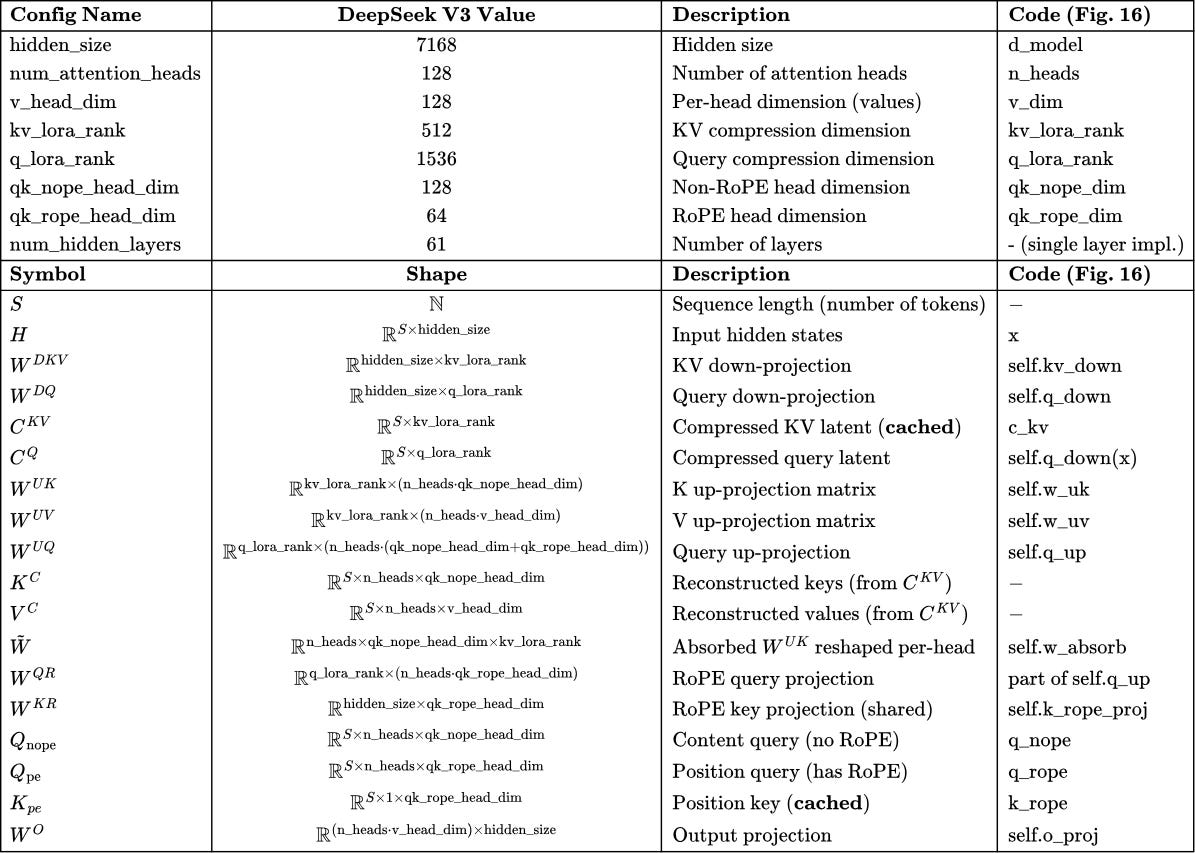
To make it more accessible to the reader, in Tab. 3 we present a high-level summary of all symbols introduced in this section alongside the example values used in the DeepSeek V3 config.

Table 3: MLA notation reference - config parameters with DeepSeek V3 values, weight matrices with their shapes, and corresponding code variables in Fig. 16.

How does MLA work? To see where the savings come from, let’s start from standard attention. Given the input sequence of S tokens:

\(H \in \mathbb{R}^{S \times \text{hidden_dim}}\)

In normal attention, we have 4 trainable weight matrices

\(W^Q \in \mathbb{R}^{\text{hidden_dim} \times \text{head_dim} \times \text{num_attention_heads}}\)

\(W^K \in \mathbb{R}^{\text{hidden_dim} \times \text{head_dim} \times \text{num_kv_heads}}\)

\(W^V \in \mathbb{R}^{\text{hidden_dim} \times \text{head_dim} \times \text{num_kv_heads}}\)

\(W^O\in \mathbb{R}^{\text{hidden_dim} \times \text{hidden_dim}}\)

For the attention equation itself, we calculate three projections:

\(Q = H W^Q, \quad K = H W^K, \quad V = H W^V\)

\(S \text{ is the sequence length}\)

\(\mathbf{Q} \in \mathbb{R}^{S \times \text{head_dim}}\)

\(\mathbf{K} \in \mathbb{R}^{S \times \text{head_dim}}\)

\(\mathbf{QK}^T \in \mathbb{R}^{ S \times S}\)

\(\mathbf{V} \in \mathbb{R}^{S \times \text{head_dim}}\)

\(\mathbf{QK}^T\mathbf{V} \in \mathbb{R}^{S \times \text{head_dim}}\)

The core idea behind MLA is that instead of caching full keys and values, we compress them into a shared latent representation - and only this representation is cached.

We have a KV down-projection (compression) matrix:

\(W^{DKV}\in \mathbb{R}^{\text{hidden_dim} \times \text{kv_lora_rank}} \)

We apply this matrix to H producing a compressed latent matrix

\(C^{KV} = H W^{DKV} \in \mathbb{R}^{S \times \text{kv_lora_rank}} \tag{7}\)

The main benefit of this compression is that kv_lora_rank is significantly smaller than what we’d need to cache storing full keys and values.

\(\text{kv_lora_rank} \ll (\text{num_attention_heads}\times \text{head_dim})\)

E.g., in the case of DeepSeek:

\(\text{kv_lora_rank} = 512 \quad \text{vs.} \quad \text{num_attention_heads} \times \text{head_dim} = 128 \times 128 = 16{,}384\)

or ~3% of the potential memory footprint had MHA been used.

Keys and values can be reconstructed from C^KV by applying the up-projection matrices W^UK and W^UV:

\(K^C = C^{KV} W^{UK} \in \mathbb{R}^{S \times (\text{num_attention_heads} \times \text{head_dim})}, \quad V^C = C^{KV} W^{UV} \in \mathbb{R}^{S \times (\text{num_attention_heads} \times \text{head_dim})} \tag{8}\)

where:

\(W^{UK}, W^{UV} \in \mathbb{R}^{\text{kv_lora_rank} \times (\text{num_attention_heads}\times \text{head_dim})}\)

The algebraic trick: absorbing matrices

Matrix multiplication is associative, meaning:

\((AB)C = A(BC)\)

This allows us to precompute and “absorb” projection matrices, avoiding the need to explicitly reconstruct keys during inference.

We can also compress queries using a down projection matrix:

\(W^{DQ} \in \mathbb{R}^{\text{hidden_dim} \times \text{q_lora_rank}}\)

We apply this matrix to H producing a compressed query latent matrix:

\(C^Q = H W^{DQ} \in \mathbb{R}^{S \times \text{q_lora_rank}}\)

Queries can be reconstructed from the matrix C^Q by applying the up-projection matrix W^UQ:

\(Q^C = C^Q W^{UQ}\)

where:

\(W^{UQ} \in \mathbb{R}^{\text{q_lora_rank} \times (\text{num_attention_heads} \times \text{head_dim})}\)

Note: In DeepSeek config (Fig. 13), q_lora_rank = 1536 while kv_lora_rank = 512, so queries use a larger latent dimension than KV, which makes sense since queries aren’t cached during decode anyway.

Now consider the attention score computation:

\(\mathbf{QK}^T \in \mathbb{R}^{ S \times S}\)

or in MLA notation:

\(Q^C (K^C)^\top = (C^Q W^{UQ})(C^{KV} W^{UK})^\top\)

Expand the transpose:

\(\begin{aligned} Q^C (K^C)^\top &= C^Q W^{UQ} (W^{UK})^\top (C^{KV})^\top \\ &= C^Q \underbrace{W^{UQ} (W^{UK})^\top}_{\tilde{W} \in \mathbb{R}^{\text{q_lora_rank} \times \text{kv_lora_rank}}} (C^{KV})^\top \end{aligned} \tag{9}\)

We never need to explicitly compute K^C! The up-projection W^UK gets absorbed into a precomputed matrix W~.

This is the key computation advantage that significantly boosts the performance. We calculate W~ only once and reuse for all computations. We multiply it with the compressed query latent matrix and compressed (kv) latent matrix.

Algebraically, the same trick can be applied to values and output projections. After computing attention weights A = softmax(Q^C (K^C)^T), we could compute:

\(O = A \cdot V^C \cdot W^O\)

Substituting V^C = C^KV W^UV:

\(O = A \cdot C^{KV} W^{UV} \cdot W^O\)

By associativity:

\(O = A \cdot C^{KV} \cdot \underbrace{W^{UV} W^O}_{\tilde{W}^{VO} \in \mathbb{R}^{\text{kv_lora_rank} \times \text{hidden_dim}}}\)

However, unlike the K absorption, this fusion is not done in practice. As shown in Tab. 4, the fused W~^VO would be 3.7x larger than keeping W^UV and W^O separate:

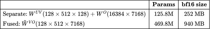
Table 4: Parameter count and memory footprint of separate vs fused value/output projections. Fusing W^UV W^O would eliminate one matmul but increases weight size 3.7x, making it impractical for memory-bound decode.

Because of this extra footprint, in practice SGLang and vLLM apply W^UV and W^O as two separate operations after attention. Only the K absorption W~ = W^UQ (W^UK)^T is precomputed at warmup.

The RoPE Problem

Modern LLMs use Rotary Position Embeddings (RoPE), which encode position information by rotating the query and key vectors. The rotation depends on the token’s position in the sequence.

Mathematically, RoPE applies position-dependent rotations

\(Q_{\text{RoPE}} = \text{RoPE}(Q), \quad K_{\text{RoPE}} = \text{RoPE}(K)\)

Let’s see what happens when we try to apply the absorption trick with RoPE. If we naively apply RoPE to the reconstructed keys and queries:

\(Q^C_{\text{RoPE}} = \text{RoPE}(C^Q W^{UQ})\)

\(K^C_{\text{RoPE}} = \text{RoPE}(C^{KV} W^{UK})\)

Problem: We’re forced to materialize the full K^C = C^KV W^UK in order to apply RoPE to it. The absorption trick no longer works - we can’t precompute W~ = W^UQ(W^UK)^T when RoPE sits in between:

\(Q^C_{\text{RoPE}} (K^C_{\text{RoPE}})^T = \text{RoPE}(C^Q W^{UQ}) \cdot \text{RoPE}(C^{KV} W^{UK})^T\)

The solution? Decoupled RoPE - split the attention into two parts:

Part 1: Content attention (compressed, no RoPE)

• Captures semantic similarity between tokens

• Lives in compressed space - absorption works perfectly

Part 2: Position attention (small, has RoPE)

• Captures positional relationships

• Small additional dimension - compute directly without absorption

Concretely, we split queries and keys into nope (no position embedding) and rope components (Tab. 5):

Table 5: The two components of MLA’s decoupled attention. Content (nope) lives in compressed space where absorption works. Position (rope) is computed directly in a small additional dimension.

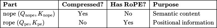
The nope Part (Content)

The content components come from our compressed latents, exactly as before:

\(Q_{nope} = C^Q W^{UQ}_{nope} \in \mathbb{R}^{S \times \text{num_attention_heads} \times \text{qk_nope_head_dim}}\)

\(K_{nope} = C^{KV} W^{UK}_{nope} \in \mathbb{R}^{S \times \text{num_attention_heads} \times \text{qk_nope_head_dim}}\)

Where:

\(W^{UQ}_{nope} \in \mathbb{R}^{\text{q_lora_rank} \times (\text{num_attention_heads} \cdot \text{qk_nope_head_dim})}\)

\(W^{UK}_{nope} \in \mathbb{R}^{\text{kv_lora_rank} \times (\text{num_attention_heads} \cdot \text{qk_nope_head_dim})}\)

The absorption trick works perfectly here - no RoPE to get in the way:

\(Q_{nope} \cdot K_{nope}^T = C^Q \underbrace{W^{UQ}_{nope} (W^{UK}_{nope})^T}_{\tilde{W}_{nope}} (C^{KV})^T \tag{10}\)

The rope Part (Position)

The position components have RoPE applied, so we compute them directly:

\(Q_{pe} = \text{RoPE}(C^Q W^{QR}) \in \mathbb{R}^{S \times \text{num_attention_heads} \times \text{qk_rope_head_dim}}\)

\(K_{pe} = \text{RoPE}(H W^{KR}) \in \mathbb{R}^{S \times 1 \times \text{qk_rope_head_dim}}\)

Where:

\(W^{QR} \in \mathbb{R}^{\text{q_lora_rank} \times (\text{num_attention_heads} \cdot \text{qk_rope_head_dim})}\)

projects to all heads, and:

\(W^{KR} \in \mathbb{R}^{\text{hidden_size} \times \text{qk_rope_head_dim}}\)

projects to a single shared key.

Note the asymmetry: Q_pe is computed per-head while K_pe is shared across all heads. This is an intentional design choice by DeepSeek - the shared K_pe is broadcast to all 128 heads during attention computation.

Why this asymmetry? (Tab. 6)

Table 6: Asymmetry in MLA’s position embeddings. Per-head Q_pe allows heads to specialize in positional patterns at no memory cost. Shared K_pe saves 128x on position key cache.

This design saves 128× on the position key cache while still allowing heads to specialize in different positional patterns through their per-head Q_pe.

Combined Attention Scores

Conceptually, we can think of queries and keys as concatenations of their nope and rope parts. For each head i:

\(Q_i = [Q_{nope,i} \mid Q_{pe,i}], \quad K_i = [K_{nope,i} \mid K_{pe}]\)

This means the attention scores decompose additively:

\(\text{Scores}_i = Q_i K_i^T = Q_{nope,i} \cdot K_{nope,i}^T + Q_{pe,i} \cdot K_{pe}^T \tag{11}\)

Crucially, we never actually concatenate these tensors. Instead, we compute the two terms separately:

1. Content scores: Q_nope,i * K_nope,i^T ∈ ℝ^(S × S) - computed via absorption trick using C^Q and C^KV

2. Position scores: Q_pe,i * K_pe^T ∈ ℝ^(S × S) - computed directly (small and fast)

Both terms produce an S × S matrix per head, so they can simply be added:

\(\text{Scores}_i = \text{ContentScores}_i + \text{PositionScores}_i\)

This is why MLA is efficient - we never materialize the full K_nope (of shape S x num_attention_heads x qk_nope_head_dim) during decode. The absorption trick lets us go directly from cached C^KV (of shape S x kv_lora_rank) to attention scores.

Putting it all together, in Fig. 13 we present a minimal implementation of MLA decode - the MQA mode in DeepSeek’s terminology. This is the path that runs during token generation, where absorption makes decode memory-efficient. Prefill uses a different path (MHA mode) that reconstructs full K/V and runs standard flash attention - we explain why in the Appendix.

Compare this with the GQA implementation in Fig. 8 - the key differences are:

1. Compressed KV cache (marker ❶): instead of caching separate K and V tensors of size n_kv_heads × head_dim, we cache a single compressed latent C^KV of size kv_lora_rank (Eq. 7) plus a small RoPE key of size qk_rope_head_dim. This is the source of MLA’s memory savings.

2. K absorption (marker ❷): instead of reconstructing full keys from C^KV, we reshape W^UK per-head and use it to project q_nope into the latent space (Eq. 9). The query then attends directly against C^KV without materializing full keys.

3. Decoupled RoPE (marker ❸): position information is handled separately through small additional dimensions (qk_rope_head_dim = 64), keeping the absorption trick valid for the content part (Eq. 11).

4. Separate V and O projections (marker ❹): unlike the K absorption, fusing W^UV W^O would increase weight size 3.7x, so they remain separate.

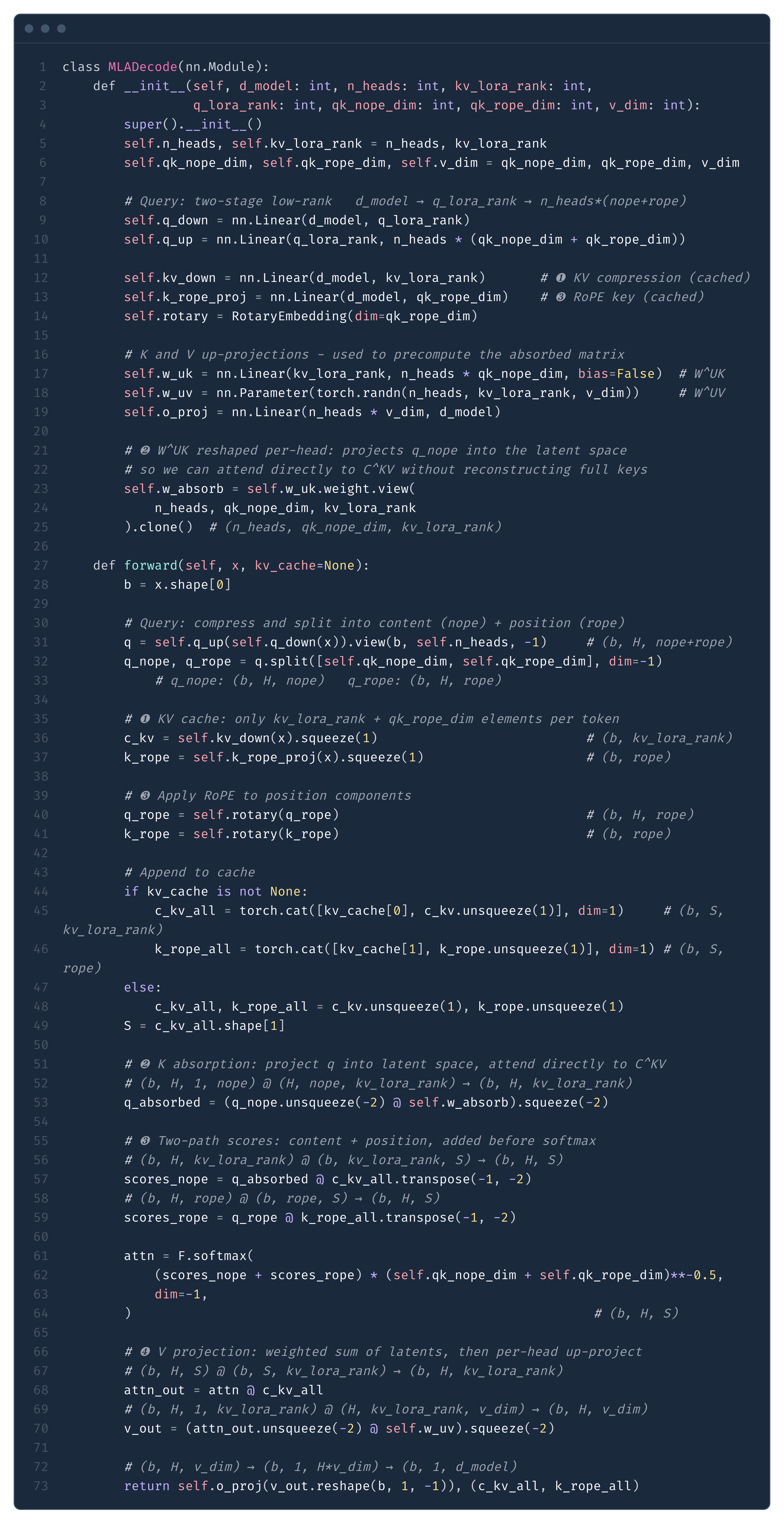
Figure 13: Minimal MLA decode implementation (MQA mode). The KV cache stores only a compressed latent C^KV (kv_lora_rank = 512) and a RoPE key (qk_rope_dim = 64) per token. Attention scores are computed via two paths: content scores through the absorbed matrix w_absorb (marker ❷), and position scores through the RoPE keys (marker ❸). Values are reconstructed per-head from C^KV via w_uv after attention (marker ❹).

Note how the KV cache stores only (c_kv, k_rope) - a compressed latent of size kv_lora_rank = 512 plus a small position key of size qk_rope_dim = 64, totalling 576 elements per token. Compare this with GQA which stores separate K and V tensors of size n_kv_heads × head_dim each. The attention computation against C^KV structurally resembles MQA - all 128 heads share the same compressed “key” - which is why MLA’s decode KV cache is so small.

KV Cache Comparison

Let’s now analyse the memory footprint reduction when MLA is used. First, we will calculate the hypothetical memory footprint of KV cache had MLA not been used, then we apply MLA optimizations and show how massively the memory is reduced. For all of the computations in this section, we will apply the numbers from the DeepSeek V3 config (Fig. 14).

Figure 14: DeepSeek V3 attention config from the HuggingFace model card. These values are used in all calculations throughout this section.

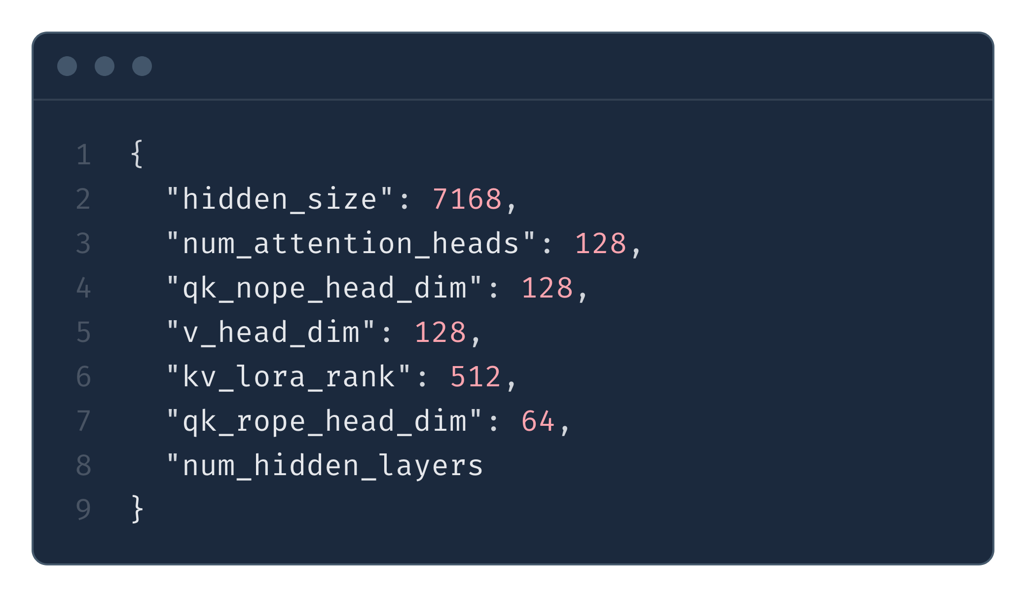
Note: DeepSeek V3’s attention dimensions (num_attention_heads × head_dim = 128 × 128 = 16384) exceed the model’s hidden_size (7168). This is possible because MLA up-projects from compressed latents. For a fair comparison, we compare against hypothetical MHA/GQA with the same attention capacity (128 heads × 128 dimensions).

In Multi-Head Attention, we cache both keys and values for all heads:

\(\text{KV Cache per token} = 2 \cdot \text{num_attention_heads} \cdot \text{head_dim} \cdot \text{num_layers}\)

\(= 2 \cdot 128 \cdot 128 \cdot 61 = 1,998,848 \text{ elements}\)

In bytes (bf16):

\(1,998,848 \times 2 = 3,997,696 \text{ bytes} \approx \mathbf{4.0 \text{ MB per token}}\)

If DeepSeek used GQA with the same ratio as Llama 3 models (8 KV heads for 64 query heads, i.e., 8:1 ratio), that would mean 128 query heads → 16 KV heads:

\(\text{KV Cache per token} = 2 \cdot \text{num_kv_heads} \cdot \text{head_dim} \cdot \text{num_layers}\)

\(= 2 \cdot 16 \cdot 128 \cdot 61 = 249,856 \text{ elements}\)

In bytes (bf16):

\(249,856 \times 2 = 499,712 \text{ bytes} \approx \mathbf{500 \text{ KB per token}}\)

With MLA, we only cache the compressed latent C^KV and the position key K_pe:

\(= (512 + 64) \cdot 61 = 35,136 \text{ elements}\)

In bytes (bf16):

\(35,136 \times 2 = 70,272 \text{ bytes} \approx \mathbf{70 \text{ KB per token}}\)

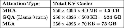
We summarize these results in Tab. 7.

Table 7: KV cache size per token across attention types, using DeepSeek V3 dimensions (128 heads, head_dim=128, 61 layers) in bf16. MLA achieves 57x reduction vs MHA and 7x vs GQA.

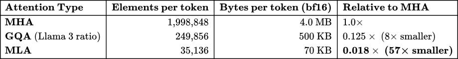
MLA achieves a 57× reduction compared to MHA, and is still 7× smaller than GQA with Llama 3’s ratio.

To put this in concrete terms, Tab. 8 shows the total KV cache at batch size 256 with 4096 cached tokens per request:

Table 8: Total KV cache memory at batch size 256 with 4096 cached tokens per request.

Figure 15: Estimated memory loaded per decode step for GQA (top) vs MLA (bottom), as a function of combined cached tokens. Both use DeepSeek V3 base dimensions (hidden=7168, 128 heads, intermediate=18432) with bf16 weights and KV cache, 61 layers. GQA uses 16 KV heads with 128-dim head (matching the Llama 3 ratio), giving 500 KB/token of KV cache. MLA stores a 512-dim compressed latent plus a 64-dim RoPE key per token, giving 70 KB/token - 7× smaller. We assume a dense MLP layer (not MoE) to stay consistent with the Llama calculations above; this does not affect the KV cache comparison which is the point of this figure.

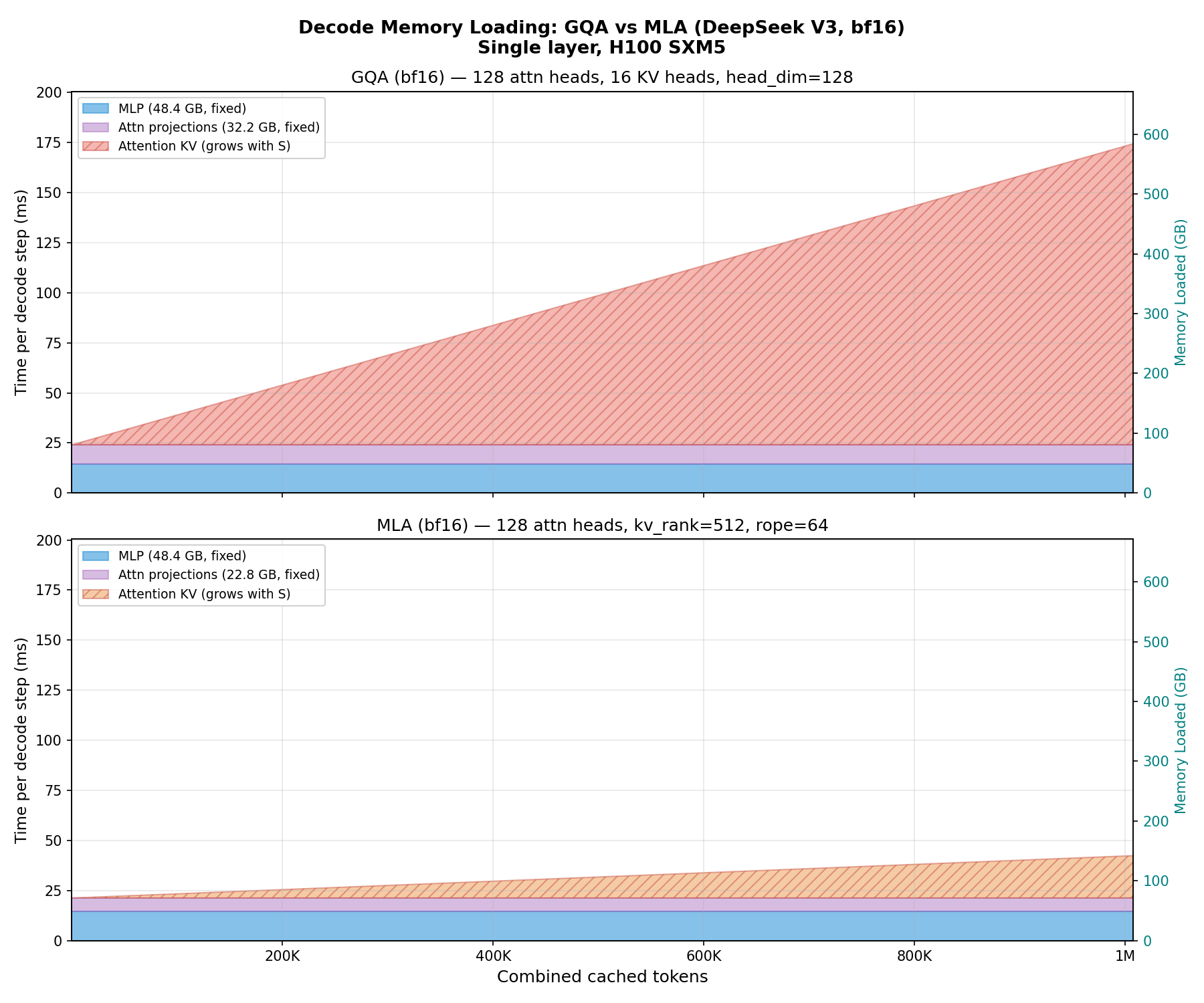
When we run these computations in real life, we observe a curve closely resembling this shape, as demonstrated in Fig. 16. We again fix the batch size at 64 and scale the sequence length. As with the GQA benchmark (Fig. 10), this is for a single transformer layer - in a full model the pattern repeats across all layers. Note that DeepSeek V3 uses MoE rather than the dense MLP we benchmark here; for the sake of simplicity we use a dense MLP as a proxy.

Figure 16: Measured MLA decode latency for one transformer layer on H100 SXM5, batch=64, DeepSeek V3 config (bf16). MLP (blue) and attention projections (purple) are fixed. MLA attention KV (red, hatched) grows linearly but much slower than GQA (Fig. 10) thanks to the compressed latent (576 elements vs 2048 for GQA). The teal dashed line shows the time predicted by dividing total memory loaded by H100 HBM bandwidth (3.35 TB/s) - the close match confirms decode remains memory-bandwidth bound. Compare with the theoretical prediction in Fig. 15. Benchmark uses FlashMLA.

DeepSeek Sparse Attention

MLA was the first attention mechanism breakthrough introduced by DeepSeek, but not the last one. In September 2025, with DeepSeek-V3.2-Exp, they introduced DeepSeek Sparse Attention (DSA). The technique is described in the DeepSeek V3.2 tech report and shares the core idea of using lightweight attention heads for token selection with Native Sparse Attention (NSA), a concurrent work from overlapping authors. DSA is built on top of MLA - the core attention mechanism stays the same, DSA just adds a selection step before it. In principle, the same idea should work with standard attention mechanisms.

Recall from the previous section that MLA dramatically compressed the KV cache (Eq. 12) - from 4.0 MB per token (MHA) down to 70 KB per token (bf16) or 35 KB per token (FP8). This was a 57× reduction. And yet, as we showed in Figure 15, even with this compression the KV cache still grows linearly with the number of cached tokens. At long enough contexts, it once again dominates the memory loading.

The insight behind DSA is: do we really need to attend to all past tokens? What if we could cheaply figure out which tokens matter, and only attend to those?

Figure 17: DSA decode flow. The lightning indexer cheaply scores all S tokens using 64 MQA heads (132 B/token), then top-k selection picks the most important k=2048 tokens. The full MLA attention (128 heads) runs only over the selected tokens (656 B/token) - identical to dense MLA, just fewer tokens.

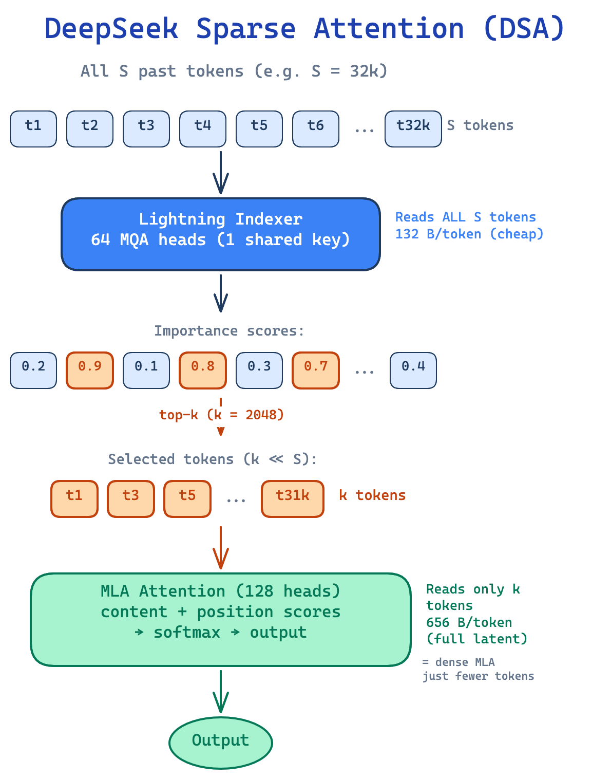
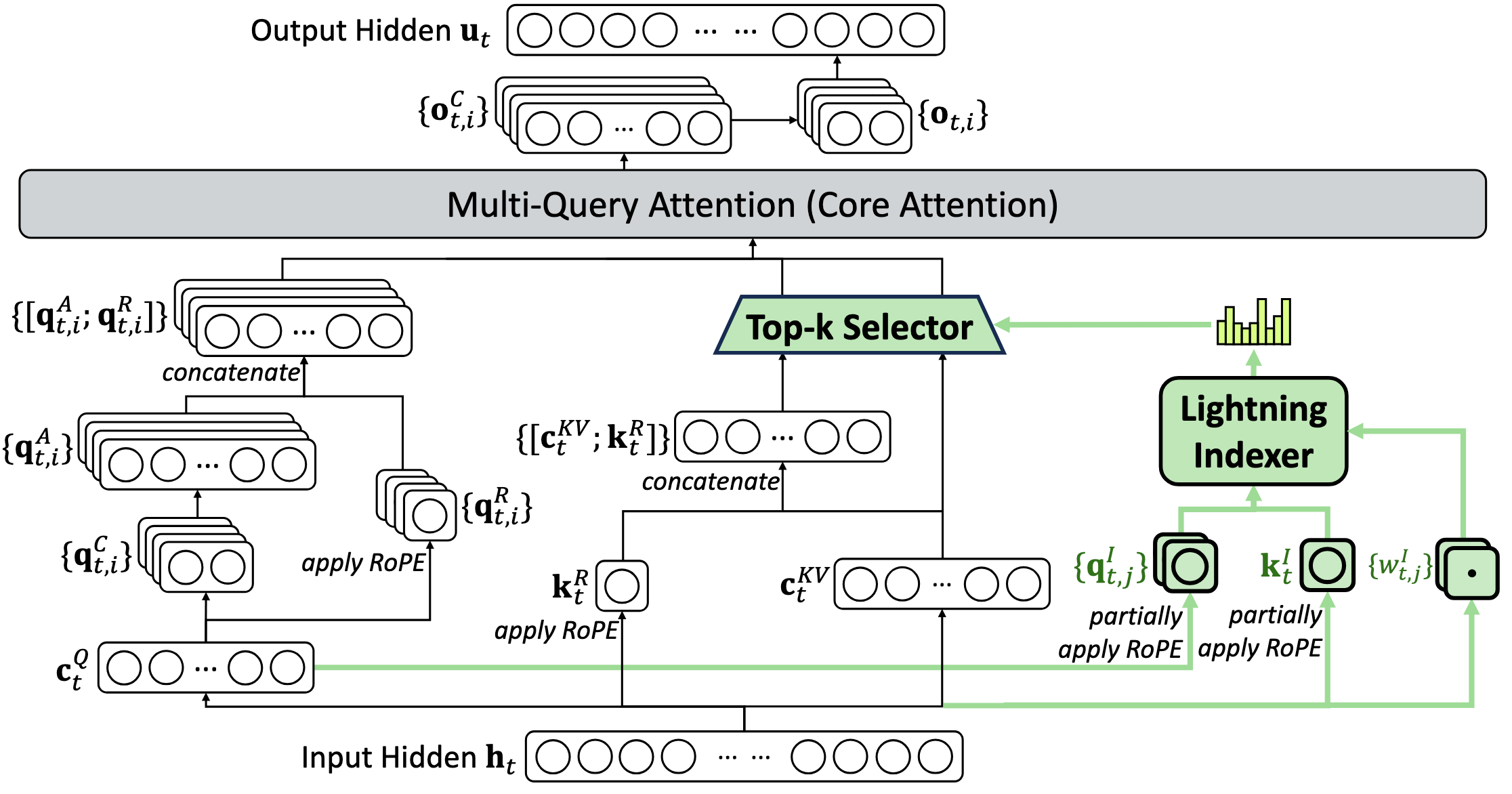
This is exactly what DSA does (Fig. 17). It introduces a lightning indexer - a small set of lightweight attention heads that score all past tokens and pre-select the k most important ones. Then the proper, expensive MLA attention is computed only over these k selected tokens.

The indexer is designed to be cheap. It uses MQA (a single shared key across all 64 heads), so its KV cache is tiny. It only computes dot-product scores - no full attention, no values. The indexer score for how relevant past token s is to the current query token t (see Fig. 17) is:

\(I_{t,s} = \sum_{j=1}^{H_I} w^I_{t,j} \cdot \text{ReLU}(\mathbf{q}^I_{t,j} \cdot \mathbf{k}^I_s) \tag{13}\)

Each of the 64 indexer heads computes a dot product between its query and the single shared key, applies ReLU (so only positive contributions count), and the results are combined via learned weights into one score per past token. The top-k scoring tokens are then selected, and standard MLA attention runs only over these k tokens - identical to dense MLA (Fig. 13), just with fewer KV entries. The full architecture is shown in Figure 18.

Figure 18: Attention architecture of DeepSeek-V3.2, where DSA is instantiated under MLA. The green part illustrates how DSA selects the top-k key-value entries according to the indexer. From DeepSeek V3.2 tech report.

Memory savings

Let’s calculate how much data DSA needs to load during decode compared to dense MLA. In the SGLang implementation, the indexer uses H_I = 64 heads with key dimension d_I = 128, and the default k = 2048.

Note that in the previous sections we calculated KV cache sizes in bf16 (2 bytes per element). From here on we switch to FP8 - the production DSA kernels (both the indexer and the sparse attention) operate in FP8, and to make a fair comparison we benchmark the dense MLA baseline in FP8 as well.

Dense FP8 MLA reads the full compressed latent for every cached token. Each token stores kv_lora_rank + qk_rope_head_dim = 576 elements. In practice, SGLang stores slightly more than 576 bytes because not all components use FP8:

• 512 bytes - compressed latent (NoPE) in FP8

• 16 bytes - FP8 per-block scale factors (4 × float32, block size 128)

• 128 bytes - RoPE key in bf16 (positional embeddings need higher precision)

This gives 656 bytes per token per layer, and we must read all N tokens:

\(\text{Dense MLA KV per layer} = N_{\text{tokens}} \times 656 \text{ bytes} \tag{14}\)

DSA has two separate KV caches to read. First, the indexer KV cache. A key reason the indexer is so cheap is that it only stores keys, not values - it does not compute full attention, it only computes dot-product scores to rank which past tokens are important. Furthermore, it uses MQA: a single shared key of dimension d_I = 128 across all 64 query heads. SGLang allocates the indexer buffer as:

• 128 bytes - single MQA key in FP8

• 4 bytes - FP8 per-block scale factor (1 × float32, block size 128)

This gives 132 bytes per token per layer - 5x less than what dense MLA stores per token. The indexer KV must be read for all N tokens:

\(\text{Indexer KV per layer} = N_{\text{tokens}} \times 132 \text{ bytes} \tag{15}\)

Second, the sparse attention KV cache. This stores the same 576-element MLA latent (656 bytes in mixed precision, as above). But crucially, we only read this for the k selected tokens:

\(\text{Sparse attn KV per layer} = k \times 656 \text{ bytes} \tag{16}\)

This is a fixed cost - it does not grow with N.

An important subtlety: DSA does not reduce KV cache storage - we still store all N tokens in GPU memory (the indexer needs to be able to score any past token, and the selected set changes every step). What DSA reduces is the amount of data read from HBM per forward pass. Since decode is memory-bandwidth bound, this is what determines the wall-clock time.

Putting it together for all L = 61 layers at N = 131K context (Tab. 9):

Table 9: Data read per decode step at 131K context. Dense MLA reads 5.2 GB of KV cache. DSA reads 1.1 GB total - 5x less - by using a cheap indexer (132 B/token) to select only 2048 tokens for full MLA attention.

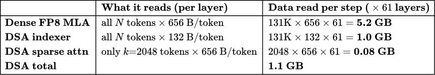
The key asymmetry: the indexer reads all N tokens but at 132 bytes each (5x cheaper per token than dense MLA). The sparse attention reads the full 656 bytes per token - but only for a fixed k = 2048 tokens regardless of context length. At 131K, DSA loads ~5x less data than dense MLA per decode step. Fig. 19 visualizes how these costs scale with context length.

Figure 19: Estimated memory loaded per decode step for different numbers of cached tokens, comparing dense FP8 MLA (top) with DSA (bottom). This calculation is done using config of DeepSeek V3 with 61 layers, assuming FP8 weights and FP8 KV cache (with bf16 RoPE). In dense MLA the KV cache grows at 40 KB/token (656 bytes × 61 layers). In DSA the memory splits into two components: the indexer KV cache grows at 8 KB/token (132 bytes × 61 layers, read for all tokens), while the sparse attention KV cache is a fixed cost of only 0.08 GB (only the top-2048 selected tokens are read, regardless of context length) - so small it is not even visible on the diagram. At long contexts, model weights dominate in DSA while KV cache dominates in dense MLA.

Real-world performance

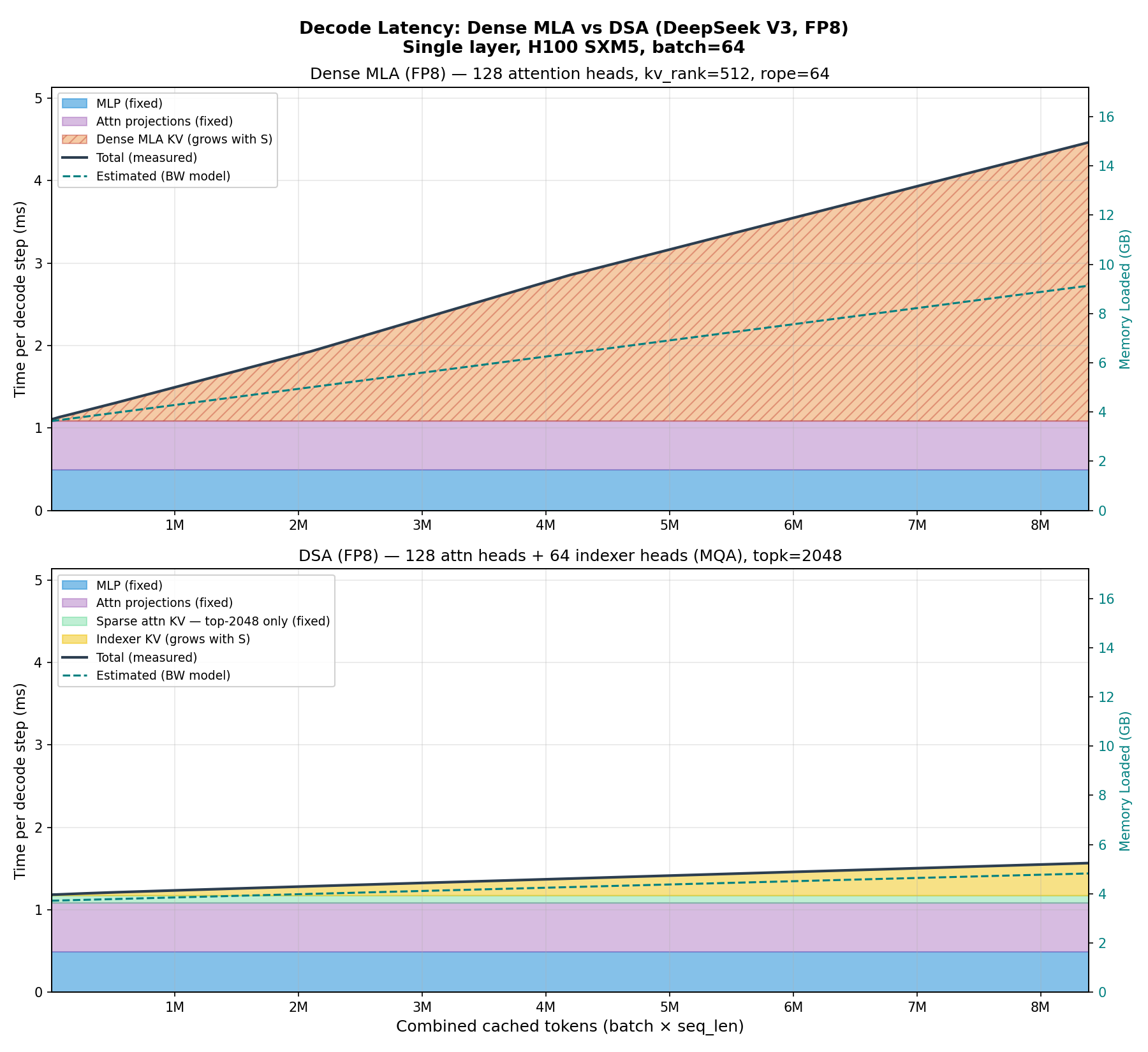
This is not just a theoretical argument. In Figure 20 we fix the batch size at 64, scale the sequence length, and measure decode latency for a single transformer layer using DeepSeek V3 dimensions. The pattern matches what we would expect from the memory analysis: the dense MLA attention cost grows linearly with context length, while DSA’s cost grows much more slowly - the sparse attention component is flat, and only the indexer grows with N.

Figure 20: Measured decode latency for one transformer layer on H100 SXM5, batch=64, DeepSeek V3 config (FP8). Top: dense MLA - attention KV (red, hatched) grows linearly with cached tokens, dominating at long contexts. Bottom: DSA - the sparse attention KV (green) is fixed regardless of context length, and only the indexer KV (orange) grows, but at 132 B/token vs 656 B/token for dense MLA. The teal dashed line shows the time predicted by dividing total memory loaded by H100 HBM bandwidth (3.35 TB/s) - the close match confirms decode is memory-bandwidth bound. Compare with the theoretical prediction in Fig. 19. Benchmark uses sgl_kernel and DeepGEMM.

Implications for MoE serving

Note that our memory loading charts above assume a dense MLP, but DeepSeek V3 uses Mixture of Experts (MoE). In DeepSeek’s production setup, each GPU manages only 2 routed experts and 1 shared expert - far smaller than the dense MLP we benchmarked. This means the MLP weight cost per forward pass is significantly smaller than what our charts show, making KV cache the dominant cost even earlier. In other words, the real-world case for DSA’s bandwidth savings is stronger than our dense-MLP figures suggest.

Beyond the raw speedup, DSA has an important implication for production MoE serving. Each GPU only holds a fraction of the experts, so at each layer tokens must be dispatched to the GPU that holds their assigned expert - requiring all-to-all communication. DeepSeek hides this cost using a dual micro-batch overlap: while one micro-batch computes, the other handles expert communication (see Figure 21). For this overlap to be efficient, the system needs to predict how long each computation phase will take. With dense MLA, the attention time varies wildly depending on the context lengths in the current batch - making it hard to design a reliable overlap schedule. DSA makes the per-layer computation time nearly constant regardless of context length (Eq. 16 - the sparse attention reads a fixed k tokens), which makes the overlap mechanism much easier to design and reason about in practice.

Figure 21: Dual micro-batch overlap schedule for DeepSeek V3 MoE inference. While one micro-batch computes (SHARED → ATTN-0 → MLP → ATTN-1), the other performs expert dispatch/combine communication in parallel. Profiling Data in DeepSeek Infra.

Minimal DSA Decode Implementation

In Fig. 22 we present a minimal implementation of DSA decode, building on the MLA decode (MQA mode) implementation above. As with MLA, prefill uses the MHA mode - reconstructing full K/V and running flash attention, with DSA adding its indexer on top (see Appendix for the prefill benchmark). The key addition for decode is the lightning indexer - a lightweight scoring mechanism that selects which tokens to attend to. The implementation highlights three properties:

1. The indexer uses MQA (❶): a single shared key across all 64 indexer heads, which is why its KV cache is so small (132 bytes/token in FP8 vs 576 bytes/token for dense MLA).

2. No values in the indexer (❷): the indexer only computes dot-product scores to rank tokens - it never does full attention.

3. Sparse attention is fixed-cost (❸): regardless of context length, the MLA attention kernel always processes exactly k tokens.

Figure 22: Minimal DSA decode implementation. Extends MLA decode with a lightning indexer that scores all S cached tokens using lightweight MQA heads (marker ❷), then selects the top-k most relevant (marker ❸). The full MLA attention runs only over the k selected tokens - a fixed cost regardless of context length.

Note how the KV cache now stores three components: the MLA compressed latent c_kv, the RoPE key k_rope, and the indexer key idx_k. During decode, the indexer scores all S tokens but only reads its small MQA keys (132 bytes/token in FP8). The MLA attention then runs over exactly topk tokens - a fixed cost regardless of how long the context grows. This is the source of DSA’s near-constant decode time.

MLA/DSA is edge-hardware friendly

A common concern with novel attention mechanisms is that they require custom GPU kernels to be practical. This is true for many architectures - writing efficient Metal, Vulkan, or even CUDA kernels is hard, and the lack of kernel support can make a mechanism unusable on edge devices like phones or laptops.

MLA (and by extension DSA) sidesteps this problem entirely. The absorption trick we described above reshapes the computation so that the decode path is just standard scaled_dot_product_attention - no custom kernel needed. This is nicely demonstrated in Fig. 23 from the MLX implementation of DeepSeek V3:

Figure 23: MLA decode in MLX (from mlx-lm deepseek_v3.py). After absorption, MLA decode is just standard SDPA - no custom kernel needed.

The key insight is that absorption converts MLA into something that structurally resembles MQA - all 128 heads share the same compressed “key” and “value” (kv_latent), and the per-head differentiation happens entirely through the query. Any framework that supports broadcasting in SDPA (PyTorch, MLX, JAX) handles this natively.

DSA adds one extra step - a gather before SDPA - which is equally portable (Fig. 24). From the MLX implementation of DeepSeek V3.2:

Figure 24: DSA decode in MLX (from mlx-lm deepseek_v32.py). DSA adds a gather before SDPA - equally portable to any framework.

Of course, production GPU kernels are significantly faster. FlashMLA fuses the two-path scores, causal mask, and attention into a single kernel. SGLang’s sparse DSA kernel fuses the gather into the attention loop, loading selected KV entries directly from HBM to SRAM without materializing an intermediate tensor. But the important point is that none of this is required - the naive SDPA path gives full correctness, full 57× KV cache compression, and the full absorption speedup, on any hardware that can do a matrix multiply.

From FLOPs to dollars

The key intuition we hope the reader gets after reading this text is that the main benefit of DSA is that as the sequence length grows, the memory footprint grows much slower (close to constant) compared to standard attention mechanism or MLA, resulting in massively improved economics of serving long-context models.

Long context is crucial for the most profitable domain of LLMs - coding assistants. DSA is the kind of architecture innovation that makes “Claude Code-like” products viable commercial projects, with positive gross margins rather than interesting demos. As SORA’s shutdown showed us, cheap economics of model serving is critical for the commercial viability of an AI product. One can have the best model capable of superhuman performance, but if the GPU math doesn’t math it won’t work as a commercial project.

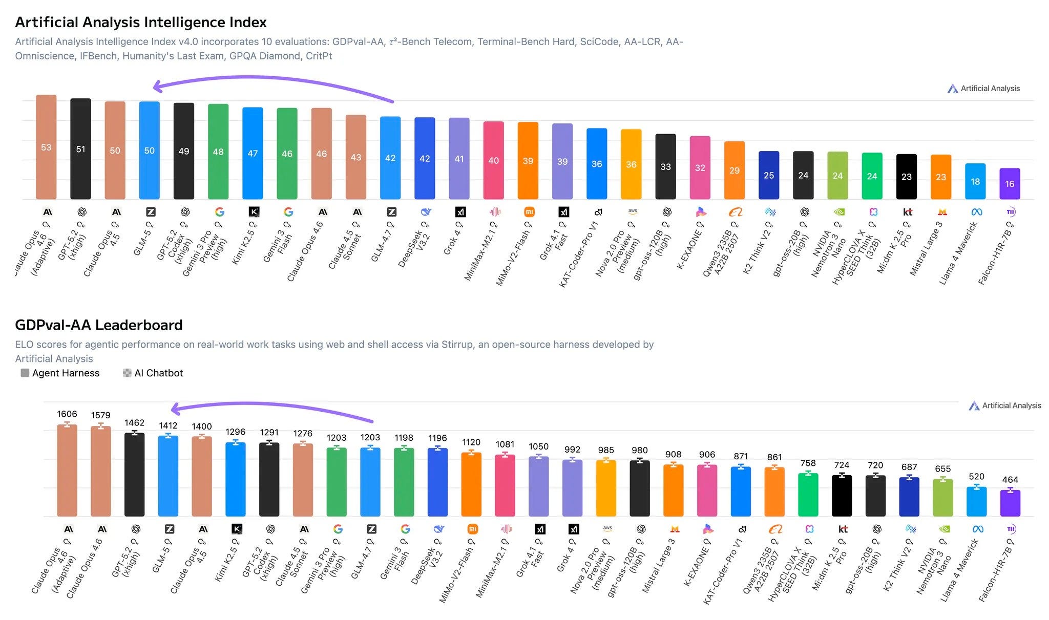
Introduction of DSA enabled DeepSeek to massively reduce the price of inference (see Fig. 2), fuelling the intelligence involution and driving down prices for other players in the space. DSA adoption seems rather slow in the industry, with one notable exception - Z.ai. The GLM5 (and its successor GLM5.1), released in 2026, utilize DSA. GLM is widely acknowledged as the leading open-source model (see Fig. 25), providing capability second only to Anthropic, Google and OpenAI (on benchmarks). The adoption of DSA by GLM5/5.1 suggests that sparse attention can be a viable alternative to standard attention.

Figure 25: Artificial Analysis Intelligence Index and GDPval-AA Leaderboard. GLM models rank among the top open-source models.

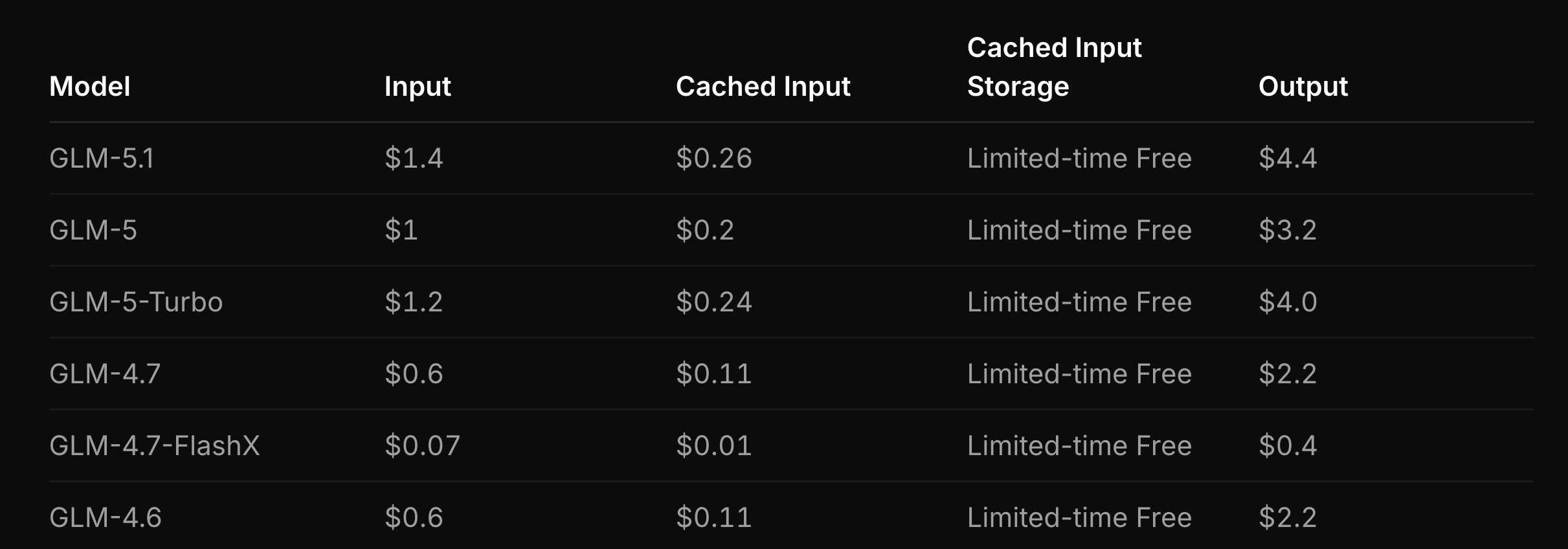
Interestingly, Z.ai’s API pricing does not pass through the efficiency gains from DSA. GLM5.1 output tokens are noticeably more expensive than GLM 4.7, and pricing has only increased with the 5.0 → 5.1 transition (see Fig. 26), despite the architectural savings from sparse attention. Part of this is justified - GLM5/5.1 has more active parameters per forward pass - but the DSA savings at long context are substantial. We interpret the higher prices and lower serving costs as a deliberate margin play: as a publicly traded company, Z.ai appears to be capturing the serving efficiency as profit rather than passing the savings onto the consumer. We expect this trend to continue - further price increases and potentially more restrictive licensing (similar to Minimax’s non-commercial license) with future releases, as the company targets significantly higher gross margins to justify the compute investment needed for next-generation of models.

Figure 26: Z.ai pricing - note that prices have only increased from 4.7 → 5.0 → 5.1, despite the move from GQA to DSA.

DSA is the key enabler of serving models cheaply at long context - a property required for any “Claude Code-like” coding assistant. Z.ai seems to be positioning the GLM Coding Plan as a key export-oriented service, a sticky product rather than a cheap commodity - one that can support revenues for the compute buildup needed for the next generation of models. Long context is of paramount importance for such a service, and DSA unlocks it. We are looking forward to the H1 2026 interim results for confirmation of this thesis.

Note: this is not investment advice. Readers should be aware that Zhipu AI is on the US Entity List, which restricts US exports to the company and may affect its long-term access to advanced hardware.

Alongside prefill caching and RLM-like scheduling of subagents to conduct sub-tasks on behalf of the main model, processing long context at scale is crucial for viability of any “Open-Claw-like” product. DSA provides the first example of a viable sparse attention mechanism that is actually working in a model at the bleeding edge. DeepSeek Sparse Attention is just the beginning - we know it works up to a 1M context window but there is no reason to believe it can’t scale further.

As we have seen in Fig. 28 for prefill and Fig. 20 for decode, the indexer becomes the bottleneck at long contexts - scaling O(S²) during prefill and O(S) during decode. There are already promising approaches to address this. GLM showed that the indexer can be shared across multiple layers, amortizing the cost. HISA takes a different approach, replacing the flat token scan with a hierarchical two-stage indexer that achieves 3.75x speedup at 64K as a training-free drop-in replacement.

Since coding agents seem to be the LLM product, there is enormous pressure on companies to improve upon sparse attention mechanisms. This, combined with how affordable it is to train - e.g. the GLM paper trains the indexer on just 20B tokens - makes us confident that DSA-like mechanisms will unlock cheap long context at the scale of millions of tokens.

One additional note: in principle, nothing prevents applying the indexer mechanism to standard attention rather than MLA. We are not aware of anyone who has tried this yet, but the sparse selection idea is orthogonal to how K and V are stored.

To sum up, we went from standard multi-head attention (MHA), through group query attention (GQA), to multi-head latent attention (MLA). We showed how the gains in each come from reducing the size of the KV cache - during the forward pass we load less data from HBM, decreasing the latency and as a result the cost of producing a token. Then we showed how DeepSeek Sparse Attention (DSA) works, examined where the savings come from, and demonstrated that this is not just a theoretical model but something observable in practice. Last but not least, we speculated on the effects of sparse attention on the economics of coding models.

Appendix

MLA Prefill: Why Absorption Doesn’t Help

The absorption trick makes decode fast - but should we use it during prefill too? The answer is no! The reason is quite simple: absorption trades smaller KV cache loading (good for memory-bound decode) for larger attention FLOPs (bad for compute-bound prefill).

During prefill there is no KV cache - we compute everything from scratch. Two options, using DeepSeek V3 dimensions: qk_nope_dim = 128, qk_rope_dim = 64, v_dim = 128, kv_lora_rank = 512, num_heads = 128.

Option 1: Reconstruct K/V (MHA mode - what real systems do). Decompress C^KV into full per-head K and V, then run standard flash attention. Each head operates on small per-head_dimensions:

\(\text{scores} = Q \cdot K^T: \quad (S \times 192) \times (192 \times S) \quad \Rightarrow \quad 2 \cdot S^2 \cdot 192 \text{ FLOPs per head}\)

where 192 = qk_nope_dim + qk_rope_dim = 128 + 64.

\(\text{output} = \text{softmax}(\text{scores}) \cdot V: \quad (S \times S) \times (S \times 128) \quad \Rightarrow \quad 2 \cdot S^2 \cdot 128 \text{ FLOPs per head}\)

Per head: 2 S^2 (192 + 128) = 2 S^2 320. Across all 128 heads:

\(\text{FLOPs}_{\text{reconstruct}} = 2 \cdot S^2 \cdot 128 \cdot 320 = 81{,}920 \cdot S^2\)

Option 2: Absorb (MQA mode - hypothetical for prefill). Skip reconstructing K/V. Instead absorb W^UK into Q (as we do in decode) and attend directly to the compressed latent C^KV. Each head now operates in the 512-dim latent space:

\(\text{content scores} = \text{q_absorbed} \cdot C^{KV,T}: \quad (S \times 512) \times (512 \times S) \quad \Rightarrow \quad 2 \cdot S^2 \cdot 512 \text{ per head}\)

\(\text{position scores} = \text{q_rope} \cdot \text{k_rope}^T: \quad (S \times 64) \times (64 \times S) \quad \Rightarrow \quad 2 \cdot S^2 \cdot 64 \text{ per head}\)

\(\text{output} = \text{softmax}(\text{scores}) \cdot C^{KV}: \quad (S \times S) \times (S \times 512) \quad \Rightarrow \quad 2 \cdot S^2 \cdot 512 \text{ per head}\)

Per head: 2 S^2 (512 + 64 + 512) = 2 S^2 1,088. Across all 128 heads:

\(\text{FLOPs}_{\text{absorbed}} = 2 \cdot S^2 \cdot 128 \cdot 1{,}088 = 278{,}528 \cdot S^2\)

The absorbed form is 3.4x more expensive (278,528 / 81,920 = 3.4). The core reason: in MHA mode each head attends in 192 dimensions (qk_nope_dim + qk_rope_dim). In MQA mode each head attends in 512 dimensions (kv_lora_rank) - the content path alone is 4x wider, and the value weighted sum also runs in 512 dims instead of 128. The projection costs are identical in both cases, so the S^2 attention term dominates at long sequences.

Since prefill is compute-bound, there is no sequence length where absorption wins for prefill. This is why SGLang (and all production engines) use MHA mode for prefill and MQA mode for decode.

Below is a minimal MLA prefill implementation matching this approach (Fig. 27):

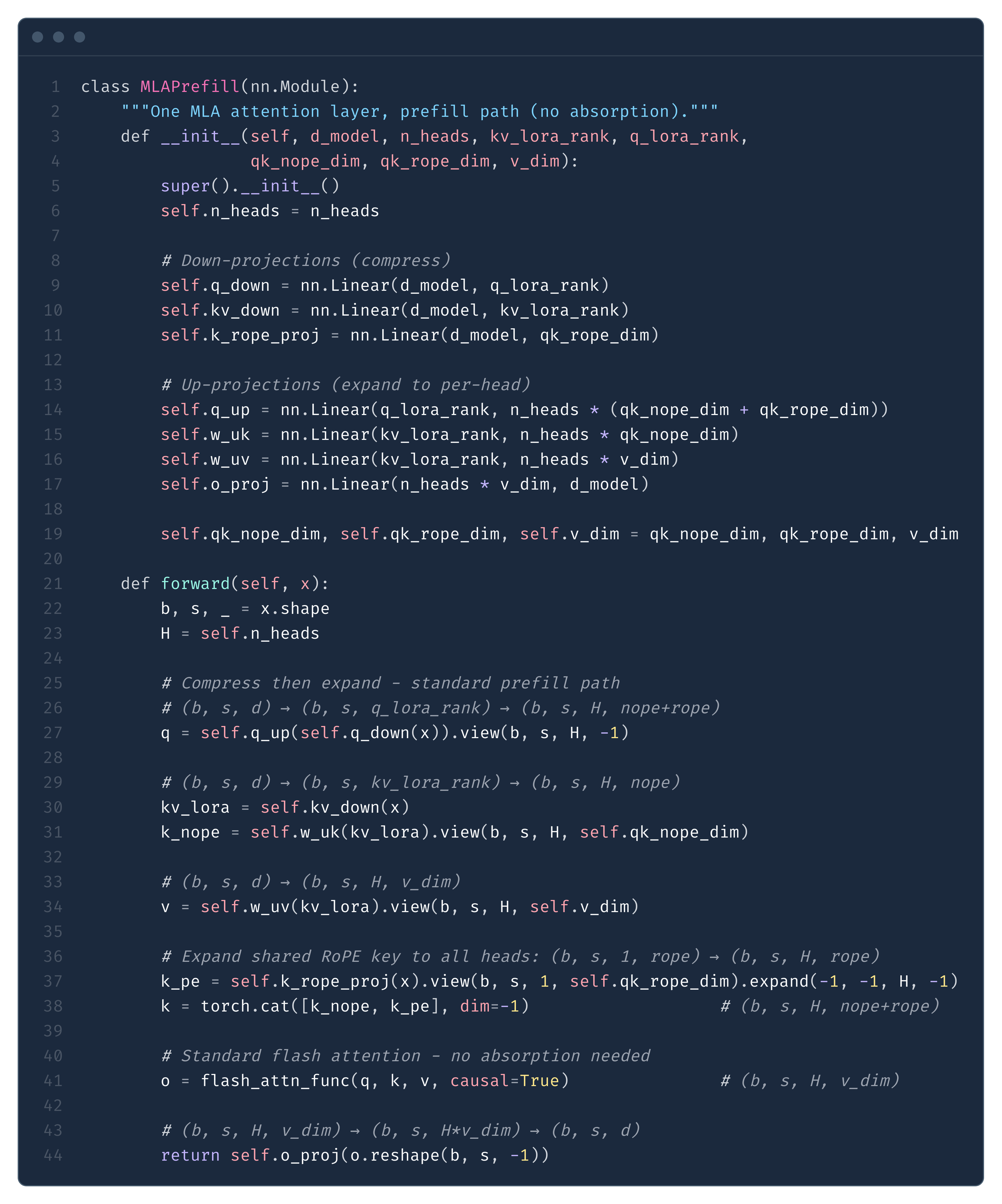
Figure 27: Minimal MLA prefill implementation (MHA mode). Unlike decode, prefill reconstructs full per-head K and V from the compressed latent via w_uk and w_uv and runs standard flash attention. This avoids the 3.4x FLOP penalty of absorption (see text above).

Note: in SGLang, q_down/kv_down/k_rope_proj are fused into one matrix (fused_qkv_a_proj_with_mqa), and w_uk/w_uv into one (kv_b_proj). RMSNorm is applied to compressed latents before up-projection, and RoPE to q_pe/k_pe. Omitted for clarity.

DSA Prefill Benchmark

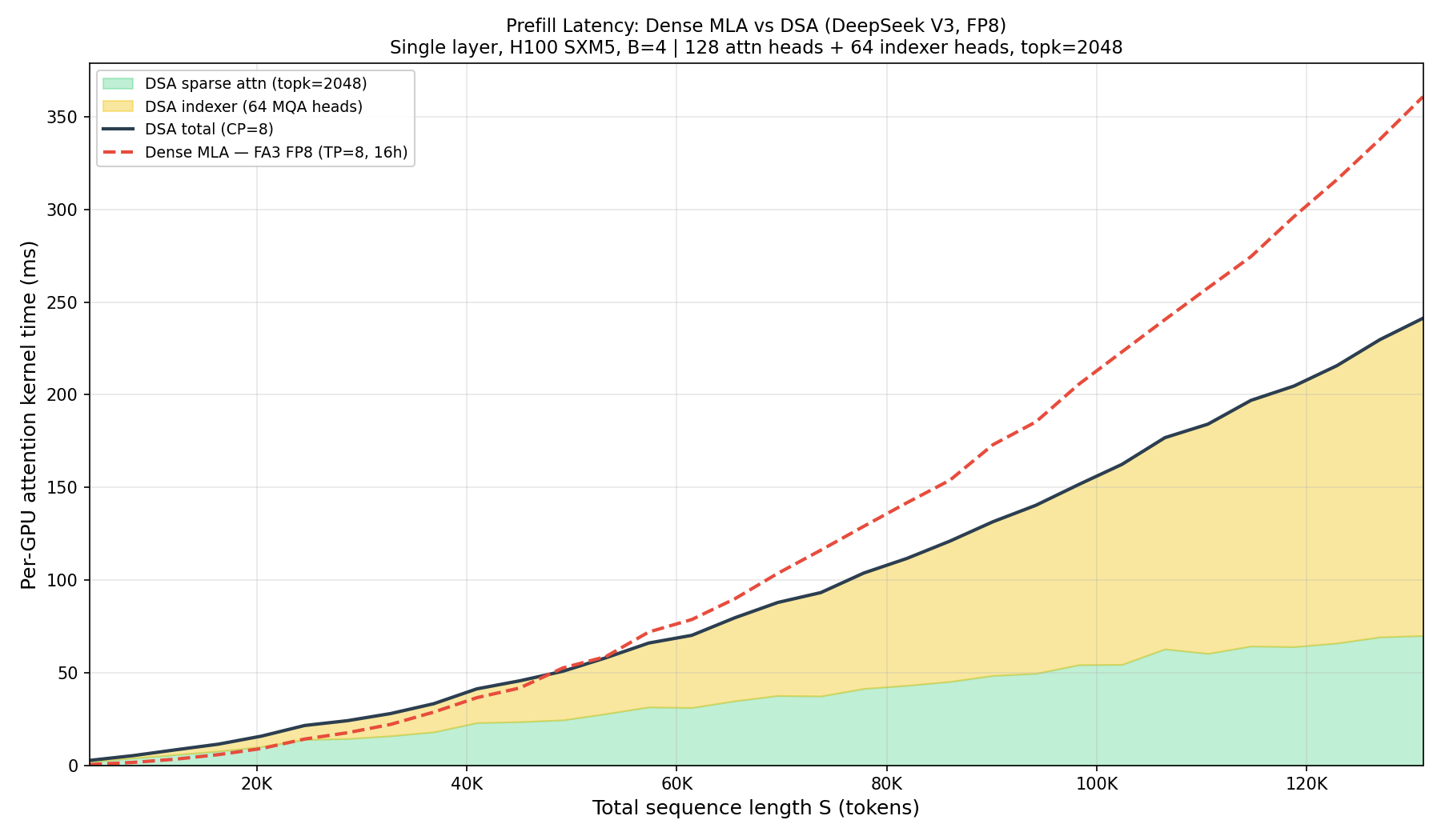
How does DSA change the prefill picture? DeepSeek’s own estimates (Fig. 1) show prefill cost growing linearly with DSA vs quadratically for dense MLA. In Figure 28 we attempt to reproduce this, comparing per-GPU prefill attention time for V3 (FA3 with tensor parallelism TP=8, 16 heads per GPU) against V3.2 DSA (context parallelism CP=8, all heads but S/8 query tokens per GPU). We use CP for DSA because the indexer can’t be split across GPUs - it needs all heads to produce a single top-k mask.

We were not fully able to replicate DeepSeek’s numbers. At short sequences DSA is actually slower than dense FA3 due to fixed overhead from the indexer and sparse kernel. DSA only pulls ahead beyond ~40K tokens, reaching 1.5x speedup at 128K. DeepSeek’s figure shows a cleaner crossover - likely reflecting differences in their production setup that we cannot reproduce with public kernels.

Note that unlike decode (where sparse attention is truly fixed-cost), during prefill both DSA components grow with S. The sparse attention grows linearly (O(S/CP × topk)), but the indexer grows quadratically (O(S²/CP)) - same scaling as FA3. DSA still wins because the indexer uses lightweight MQA heads (single shared key, 128-dim) which are much cheaper per operation than FA3’s full multi-head attention.

Figure 28: DSA prefill attention latency vs dense MLA (FA3) on a single H100 SXM5 for one transformer layer, DeepSeek V3 config (256 data points, S from 512 to 131K, B=4, topk=2048). Left: per-GPU kernel time. Right: speedup ratio - DSA becomes faster around 40K tokens and reaches 1.5x at 131K. Benchmark uses sgl_kernel, NSA Triton indexer, and DeepGEMM.

Acknowledgments

Thanks to Szymon, Pieter, Eric and Lukas for proofreading and pushing back on the parts I was confident about but shouldn’t have been.

@online{tensoreconomics2026dsa,
  author = {Piotr Mazurek},
  title = {DeepSeek Sparse Attention from First Principles},
  url = {https://www.tensoreconomics.com/p/deepseek-sparse-attention-from-first},
  urldate = {2026-04-15},
  year = {2026},
  month = {April},
  publisher = {Substack}
}