MoE Inference Economics from First Principles

DeepSeek 🐳, Kimi, synthetic data markets and the token overcapacity issue

The release of first DeepSeek R1, then Kimi K2 and then DeepSeek V3.1 mixture-of-expert (MoE) models has firmly established them as the leading architecture of large language models (LLMs) at the intelligence frontier. Due to their massive size (1 trillion parameters and up) and sparse computation pattern, selectively activating parameter subsets rather than the entire model for each token, MoE-style LLMs present significant challenges for inference workloads, significantly altering the underlying inference economics. With the ever-growing consumer demand for AI models, as well as the internal need of AGI companies to generate trillions of tokens of synthetic data, the "cost per token" is becoming an ever more important factor, determining the profit margins and the cost of capex required for internal reinforcment learning (RL) training rollouts.

This analysis examines MoE architecture through the lens of hardware limitations and costs. Key bottlenecks: FLOPS, memory bandwidth, and inter-node connection speed directly impacts end-to-end performance and user scaling potential. Building on this foundation, we develop a theoretical cost model for large-scale model serving, comparing Deepseek V3.1 and Kimi K2 and showing how the hardware costs shape the business models of LLM inference providers.

We use this world model to go from tokens to dollars - demonstrating how these models can be cost-effectively served to consumers at scale and how cheaply they can be used for synthetic data generation. We argue that this is a market opportunity currently flying under the radar and a potential growth engine for NeoClouds. Lastly, we address the elephant in the room - the surprising lack of consumption of these models. Despite the great dollar/performance ratio, the global consumption of open-source models remains surprisingly minuscule, suggesting a potential oversupply of inference providers and a capability gap that is felt by users but not necessarily reflected well in the benchmarks.

The remainder of this article proceeds as follows. We first examine DeepSeek's architecture in detail, covering multi-head latent attention (MLA), expert routing, and expert parallelism (EP). Building on DeepSeek's published optimizations—many of which are implemented in SGLang—we develop a theoretical performance model that works across diverse hardware specifications. We then validate this model against real-world performance data and use it to derive per-token pricing for different deployment configurations.

For readers seeking a concise overview of inference economics, we recommend proceeding directly to section “Hardware considerations and profit margins“, returning to examine the DeepSeek V3.1 architectural details and the theoretical model formulation as reference material when needed.

Sections “DeepSeek MoE Architecture”, “Inference Optimization Techniques” and “Throughput: Theory vs Practice” are based on the authors' work at Aleph Alpha. We publish the numbers and methods we used internally for estimating the hardware requirements and the numbers we observed through conducting experiments of running DeepSeekV3.1 on multi-node setups. The theoretical model appeared first on the Aleph Alpha Blog.

Introduction

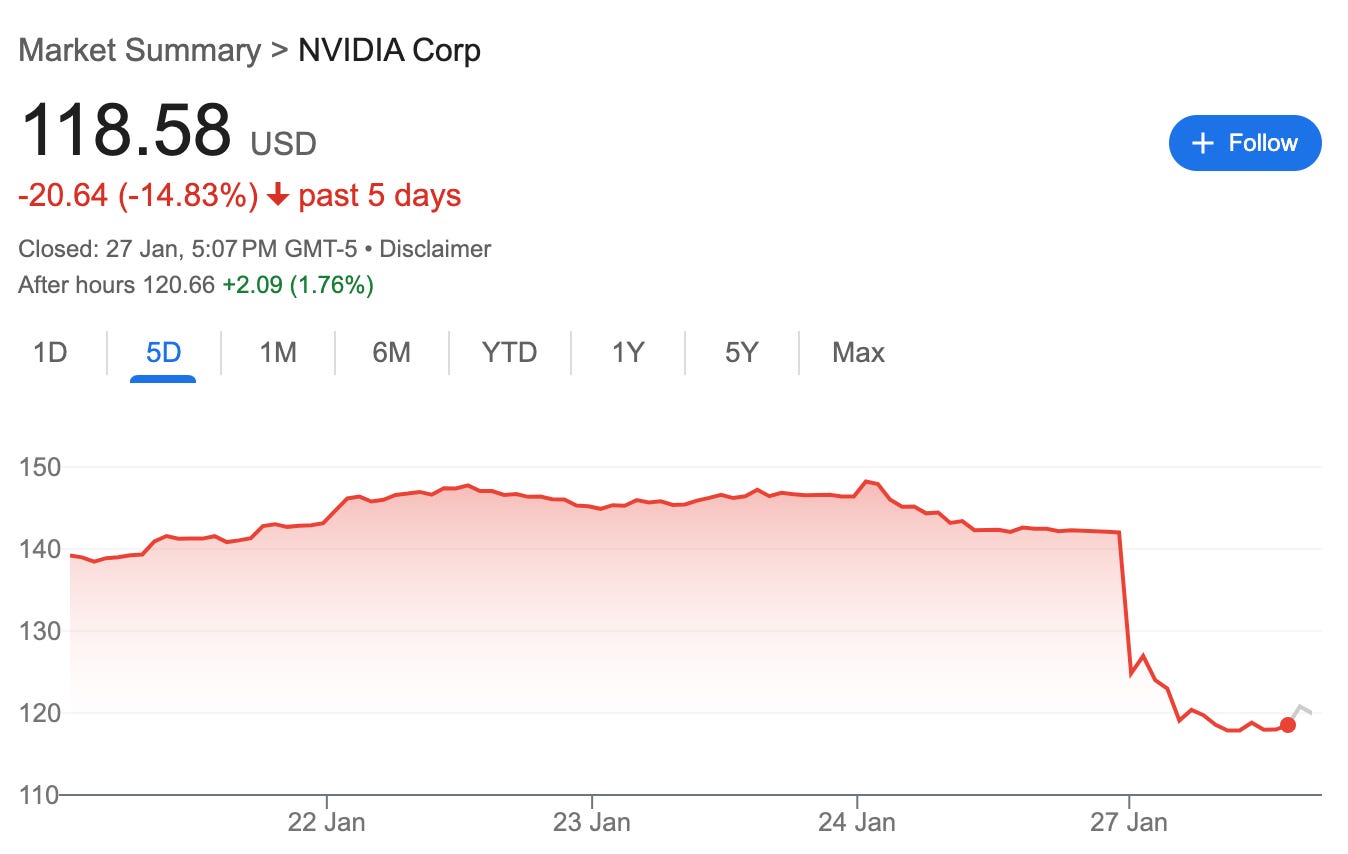
In January 2025, DeepSeek's release of their R1 reasoning model triggered the so-called "DeepSeek shock" in the global financial markets - with major Western tech companies, most notably NVIDIA (see Fig. 1), taking massive (though short-lived) losses to their market caps. While it is not possible to establish what exactly spooked the investors, it seems widely accepted that the ultimate reason was the realization of how cost-efficient it was to train the original DeepSeek V3, with the figure reported in the paper of only $5.6M, orders of magnitude less than the figures reported by various western labs.

Figure 1: The "DeepSeek moment" for NVIDIA stock price, as investors priced in the potential savings in model training.

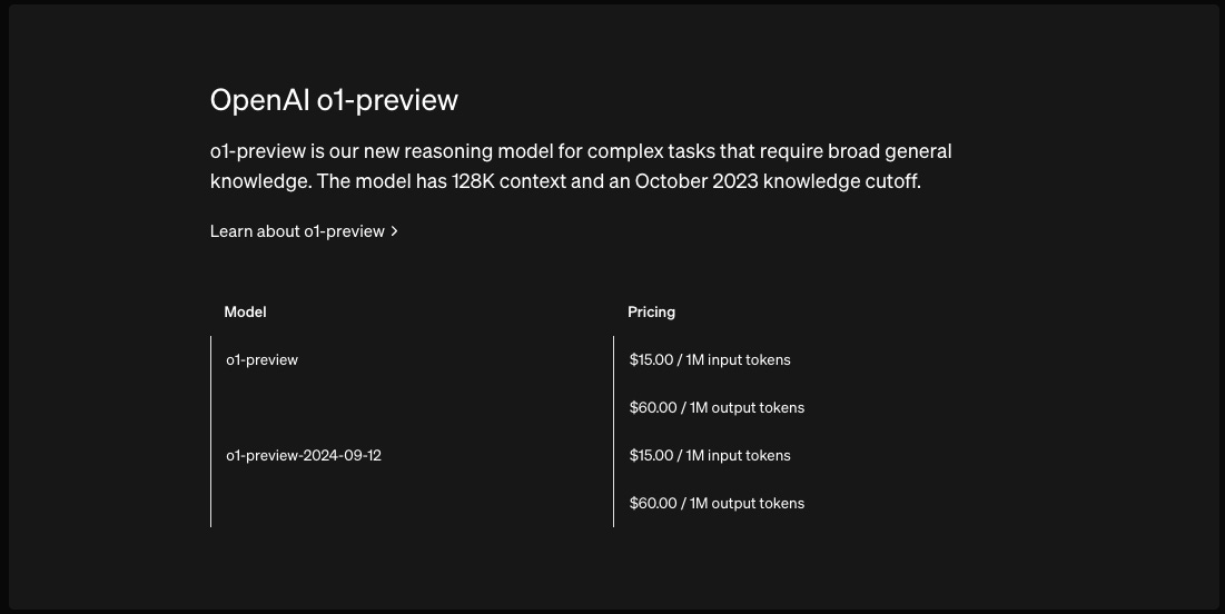
What stood out to industry insiders even more than the minuscule training budget was the massive cost advantage DeepSeek API offered. At only $2.1/1M output tokens, it provided an over 27x cost advantage (see Fig. 2) while nearly matching O1-preview's benchmark performance (the leading reasoning model at the time).

Figure 2: o1-preview pricing in January 2025, from source

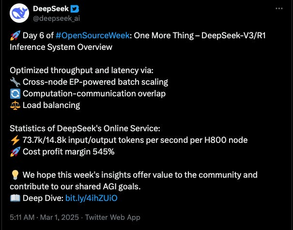
The DeepSeek team has been unprecedentedly open about the model and training details, and, most relevant to this analysis, about their inference infrastructure details. During the Open Source Week, among other things, they released efficient multi-head latent attention (MLA) kernels, an expert parallel (EP) communication library, and they published the details of their inference stack and setup, explaining the optimization techniques and releasing the theoretical revenue figures (see Fig. 3).

Figure 3: #OpenSourceWeek, when DeepSeek released their inference infrastructure details, lifting the veil on the economics behind LLM API pricing.

Understanding how DeepSeek achieved such dramatic cost advantages requires examining the underlying business model of AI inference. To quote Semianalysis here:

The modern factory is an AI token factory. Raw Silicon, electricity, and water comes into a Datacenter and what comes out is intelligence (in the form of tokens).

The business model of an 'AI token factory' is straightforward. Like any factory, there are fixed equipment costs that owners want to spread across as many users as possible. In AI inference, this fixed cost is the hourly expense of running GPUs, and providers maximize efficiency by producing as many tokens as possible per hour. The more tokens produced, the lower the cost per token - enabling cheaper pricing or higher margins. This creates a classical economics model incentivizing economies of scale: substantial fixed costs (GPU servers) that must be divided across as many users as possible.

In this article we develop a comprehensive cost model to answer one fundamental question: what does it actually cost to generate a DeepSeek V3.1 token, and what factors impact this number? We aim to build a theoretical cost model enabling us to estimate the final throughput, given the hardware specification (FLOPS, memory bandwidth, and the interconnect) and the workload profile (batch size and number of input/output tokens). We hope this will help you build a more accurate world model of this topic and make informed decisions about hardware investments and deployment strategies. We will use said theoretical model to propose the best hardware setup for deployments of different characteristics (the latency/speed/cost tradeoff).

We aim the article at experienced readers. We strongly encourage you to read and understand the core messages of “LLM Inference Economics from First Principles"first. Before proceeding to reading this article, you should be familiar with topics such as what a FLOP is, what it means to be compute/memory bound, what a KV cache is and how to calculate its memory footprint, and what prefill and decode phases are. We assume the reader is familiar with said topics, and we strongly believe that without this background the topics in this text might prove challenging to understand.

DeepSeek V3.1 and Kimi K2 are two prominent examples of mixture-of-expert style models. Understanding their cost advantages requires examining how MoE economics differ from traditional dense models. The key challenge in MoE inference is that, unlike in dense models like Llama3, each processed token activates only a subset of parameters, rather than the entire model. As we learned in the previous text, the decode (or token-by-token) phase is primarily memory bound, meaning that the majority of the execution time, and as a result most of the cost associated with running the model, comes down to the time of loading the model's parameters from the global memory. This property of dense models naturally incentivized amassing a batch as big as possible and sharing the cost of loading the model parameters across as many requests as possible, aka achieving a sort of economy of scale - fixed cost shared by multiple users.

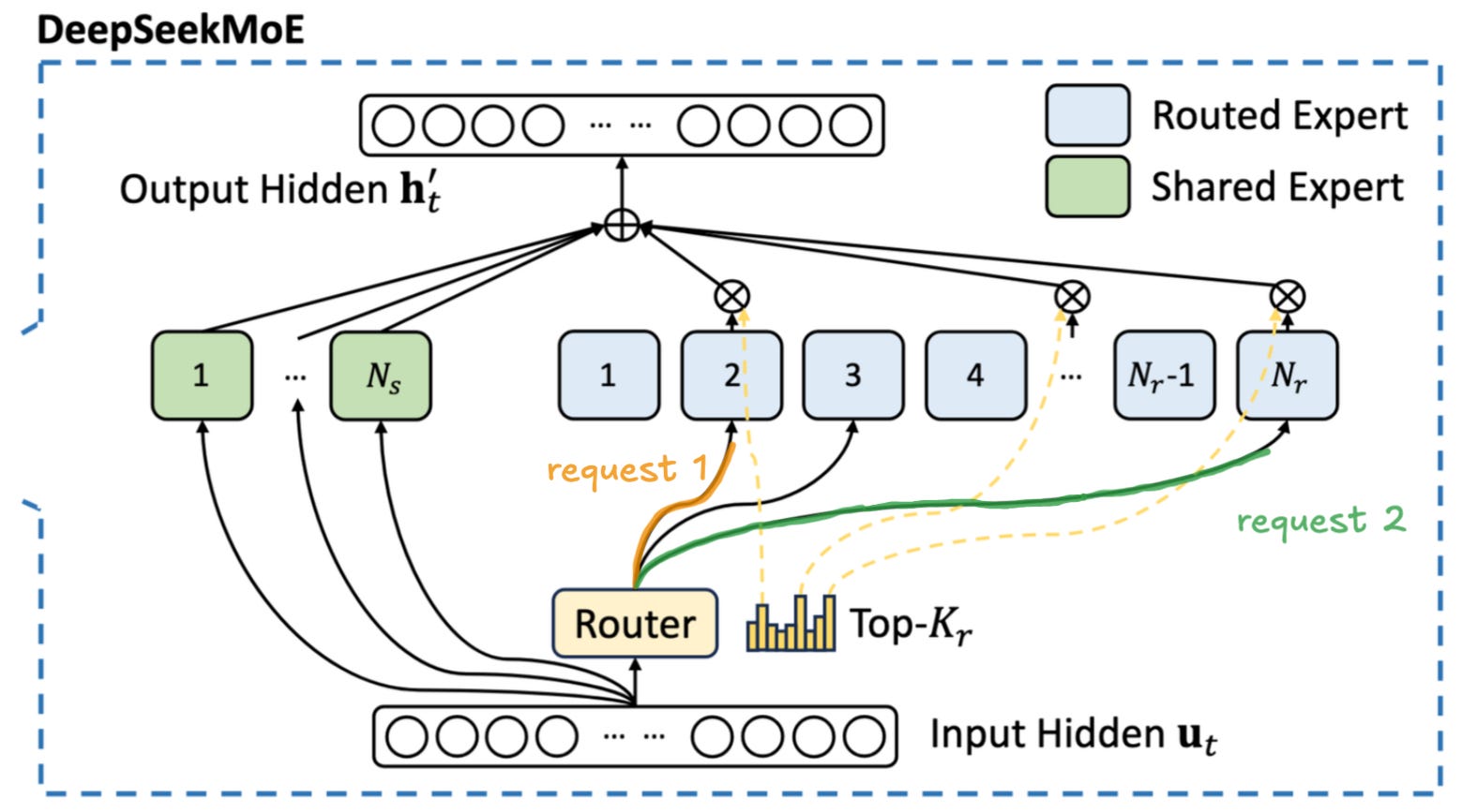
For MoEs this becomes substantially more challenging. During the decode phase, each token in the batch is activating only a small subset of parameters at every layer. This means that each request requires us to load a different part of the model, as demonstrated in Fig. 4. As the number of requests in a batch increases, a more and more substantial portion of the model will have to be loaded from global memory. The experts are chosen semi-stochastically¹, so some of the tokens in the batch will be routed to the same expert. As we progressively increase the batch size, more and more experts will be shared by different requests. This means that at the larger batch sizes we will partially recreate the situation from the dense model - sharing the cost of model loading between multiple users. Unfortunately this means that we will need significantly more requests, i.e. more users, to achieve the same "economies of scale" for MoE models.

Figure 4: Two request tokens activating different parts of the model, requiring us to load more weights, saturating the memory bandwidth

To illustrate this challenge: while DeepSeek V3.1 activates only 37B parameters for a single forward pass, this number grows nearly linearly with batch size as different queries activate different experts. At large batch sizes, the system may need to load close to the full 671B parameter model, creating severe memory bandwidth bottlenecks. Furthermore, this need for bigger batches requires substantially more resources to store the KV cache for all of the requests. These two factors necessitate running the model beyond a single node. To put it simply, there is not enough memory bandwidth, and there might not be enough space in memory on a single node to amass enough users to make model serving economically viable.

A GPU node is a specialized computer system designed with high-performance computation in mind. It is essentially a server with multiple GPUs, alongside hardware like CPUs, memory, or networking equipment. A popular example of a node would be a DGX system by NVIDIA, containing eight high-end GPUs (such as H100s, H200s, or B200s) in a single chassis, along with high-speed interconnects between the GPUs (NVLink). Within the node, the GPU-to-GPU (Intra-node) communication is possible at much higher speeds than the communication between the nodes (inter-node).

To effectively host large scale MoE-style models, an inference provider needs multiple GPU nodes. Ideally, we would like to split the model so that each GPU handles some subset of the experts and routes all relevant queries to this GPU. This way each GPU stays busy, and the GPUs do not need to communicate intermediate results as in tensor parallel (TP) setups². This approach is called expert-parallelism (EP). Note that expert choosing occurs at every layer, for every token. During the decode phase, as the model generates token after token, the new token is routed to different experts, located on different GPUs.

To quote DeepSeek themselves:

Due to the large number of experts in DeepSeek-V3/R1—where only 8 out of 256 experts per layer are activated—the model’s high sparsity necessitates an extremely large overall batch size. This ensures sufficient batch size per expert, enabling higher throughput and lower latency. Large-scale cross-node EP is essential.

As we have adopted prefill-decode disaggregation architecture, we employ different degrees of parallelisms during the prefill and decode phases:

Prefilling Phase [Routed Expert EP32, MLA/Shared Expert DP32]: Each deployment unit spans 4 nodes with 32 redundant routed experts, where each GPU handles 9 routed experts and 1 shared expert.

Decoding Phase [Routed Expert EP144, MLA/Shared Expert DP144]: Each deployment unit spans 18 nodes with 32 redundant routed experts, where each GPU manages 2 routed experts and 1 shared expert.

Increasing the number of nodes operating within a single setup has a beneficial effect not only on the end-to-end performance but also on the per node performance. In other words, we get an increased return on investment (ROI) on our fixed cost of hardware (aka GPUs). This benefit is clearly demonstrated in one of the blog posts by Perplexity (see Fig. 5). You can see that as we increase the number of nodes involved (the EP number), the per node performance increases. We can compare it to a factory - investing more money into automation tools increases the returns on the tools the factory already owns. It has a compounding effect driving down the price per token as we increase the number of nodes in a setup, but it comes at a cost - we need substantially larger usage to utilize the setup.

Figure 5: Throughput per node by Perplexity.

While running a model in the multi-node setup in theory provides enormous economies of scale, enabling the running of bigger batches far more productively, running such an operation at scale is a highly sophisticated endeavor. It requires a mature software stack and an in-depth understanding of the underlying hardware by the people involved in developing such a stack. It is clearly reflected when we look at the list of people involved in the first open-source reproduction of a multi-node DeepSeek setup by SGLang (see Fig. 6). And while there exists an open-source reproduction, as of September 2025 it is still pretty hard to operate, requiring careful coordination of different package versions and branches of underlying software libraries. We are aware of a few public inference providers who, due to the reasons above, went with serving DeepSeek on a single H200 or B200 node. While this setup is far from optimal, it is far easier to maintain and provide it to clients.

Figure 6: List of people involved in the enabling the multi-node DeepSeek setup. SGLang blopost

DeepSeek MoE Architecture

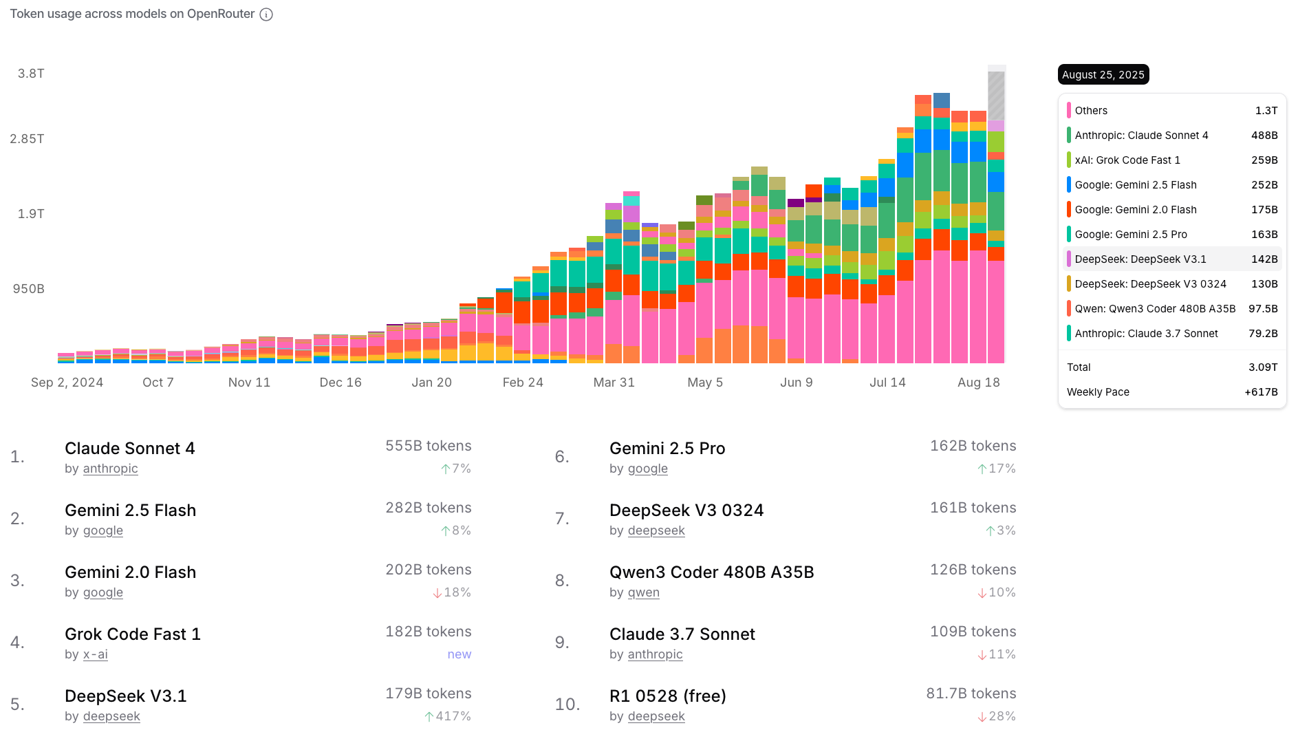
Since the "DeepSeek moment" was the motivation for us to write this article, and DeepSeek V3.1 as of September 2025 remains the most popular open-source model according to OpenRouter (see Fig. 7), we will use it as a reference architecture we use in our calculations. All DeepSeek V3, DeepSeek R1, and DeepSeek V3.1 share exactly the same architectural details; they "only" differ by the values of weights and by their behavior during inference.

DeepSeek V3.1 is a hybrid model that, depending on the inference setting, produces thousands of so-called reasoning tokens before giving a final answer. The underlying inference math is the same at the per-token layer regardless of the setting, but due to potentially vastly different distributions of input to output tokens, the inference math we will achieve will be highly dependent on whether the model is used in the reasoning or non-reasoning mode, as it is reflected by the DeepSeek pricing page (see Fig. 32).

Figure 7: OpenRouter model popularity ranking, showing DeepSeekV3.1 as the most widely used open-source model, with the old DeepSeek V3 0324 remaining a close second (30.08.2025)

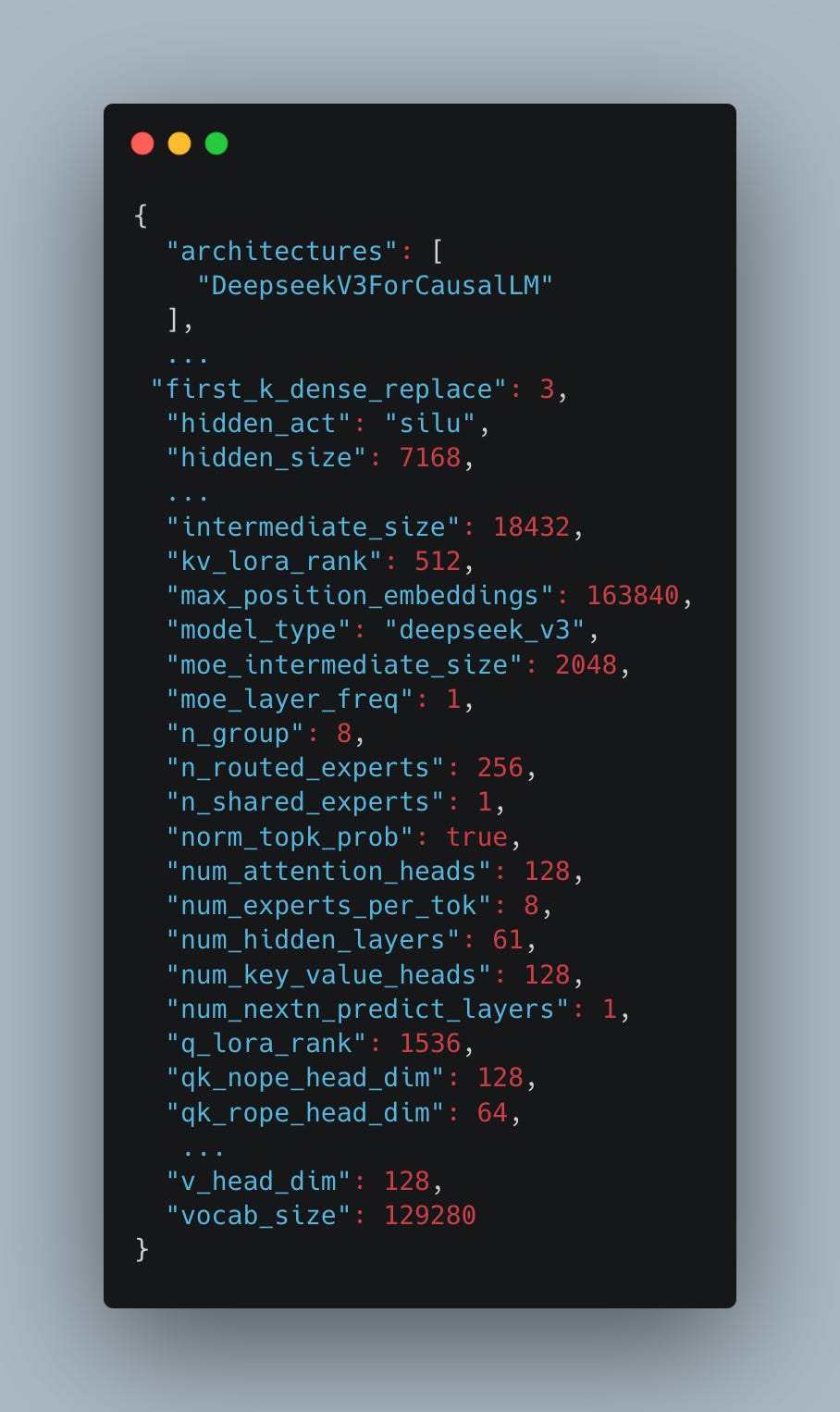
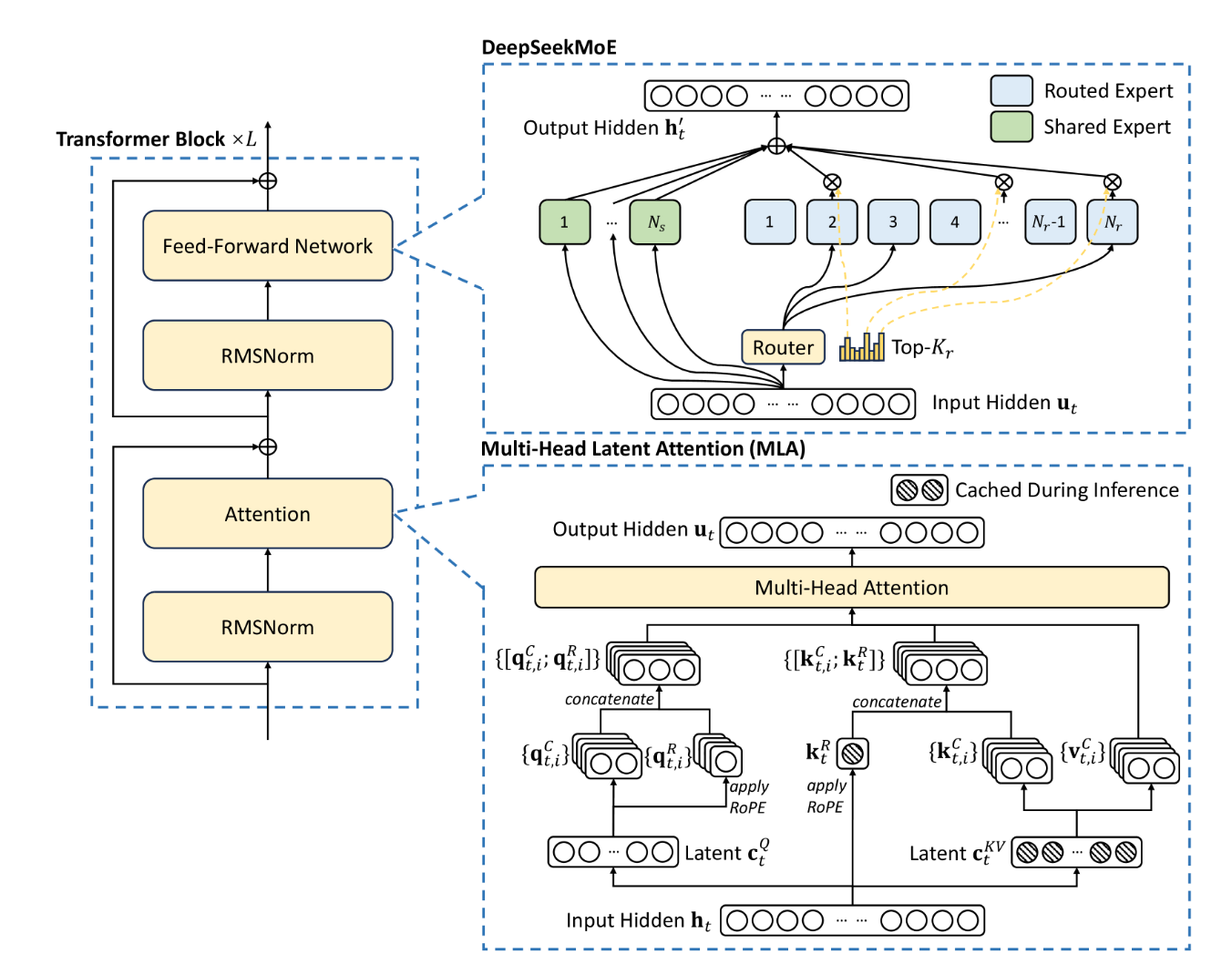
The DeepSeek architecture is summarized by the model configuration available on Hugging Face (see Fig. 8). It consists of 61 layers (num-hidden-layers), three of which are dense (first-k-dense-replace), and the remaining 58 are MoE layers. Each MoE layer contains a modified self-attention mechanism (multi-head latent attention, or MLA), a gating mechanism, and 257 experts - 1 shared expert and 256 routed experts - as defined by the n-shared-experts and n-routed-experts. The MoE layers are followed by a traditional language modeling (LM) head. The DeepSeek team also proposed a multi-token prediction (MTP) head for speculative decoding. However, as modeling its real-world performance is complex and less relevant for larger batches, we exclude it from this analysis.

Figure 8: DeepSeekV3 Hugging Face configuration. Note that this is the exact same configuration as used in DeepSeek V3 and DeepSeek R1.

Each layer consists of a Multi-head Latent Attention (MLA) followed by a DeepSeekMoE, as illustrated in Figure 9. MLA is a variant of traditional attention that compresses the KV cache using a linear algebra optimization. Instead of storing full key-value pairs like other models (such as Llama, Qwen, etc.), MLA stores only a compressed latent representation of size kv-lora-rank + qk-rope-head-dim. This reduces memory bandwidth requirements during token-by-token decoding, since less KV cache memory needs to be loaded to produce each token.

These optimizations compress the KV cache to 70KB per token - a 2-7x reduction compared to other models (Qwen3 32B: 163KB, Llama 405B: 516KB per token). This compression directly translates to reduced memory bandwidth requirements and lower inference costs. We detail the computational mechanics of MLA later; the key insight is that this architectural choice fundamentally alters the economics of serving large language models, especially with long context (such as agentic) use cases.

Following the MLA is the DeepSeekMoE component (see Fig. 9). The routing mechanism uses a linear layer mapping from hidden-size to n-routed-experts to classify which experts are most relevant for each token based on its semantic content. Each token is individually routed to a different set of experts. It is a common confusion that the experts are selected at the sequence (or query) level; we want to highlight that this is not the case. DeepSeek selects the top eight experts per token, with routing scores serving as weights when combining expert outputs.

Each expert contains a standard MLP structure with SwiGLU activation: three linear layers (W1 and W3: hidden-size → moe-intermediate-size, W2: reverse). Crucially, the moe-intermediate-size (2048) is smaller than hidden-size (7168) - the opposite of traditional dense models like Llama 3.3 70B, where intermediate dimensions are 3.5x larger (28672 vs 8192). This compression reduces per-expert computational costs while maintaining model capacity through expert diversity.

Beyond the eight routed experts, every token also passes through a shared expert that provides base knowledge common to all inputs. This hybrid approach balances specialization with computational efficiency.

This architecture is repeated across all 58 MoE layers, followed by the LM head for next-token prediction. The key architectural innovations - MLA for memory efficiency and sparse expert activation - represent a fundamental shift from traditional dense transformers toward economically optimized inference. In the following sections, we analyze the computational details of MLA and MoE components, identifying the primary bottlenecks that determine serving costs and scaling limits.

If you are not interested in the architecture details and optimizations, and you just want to read the conclusions and meta analysis feel free to skip to section "Hardware considerations and profit margins".

Figure 9: DeepSeek V3 MoE transformer layers consist of 3 shared experts and 256 routed experts. The router, a single weight matrix, predicts scores where the top 8 scores are chosen and the token is routed to the corresponding expert. In total a token goes through 9 out of 257 (256 routed + 1 shared) experts in each forward pass. Figure taken from DeepSeek V3.

Inference Optimization Techniques

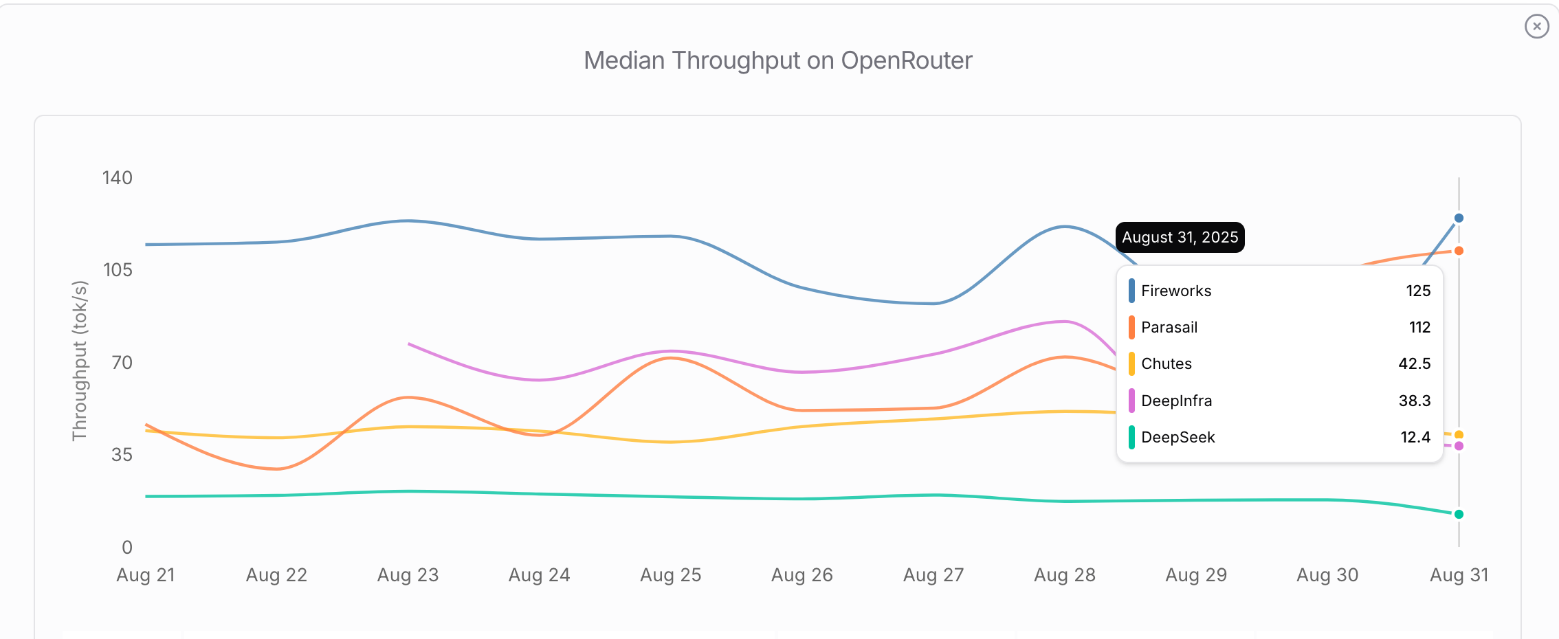
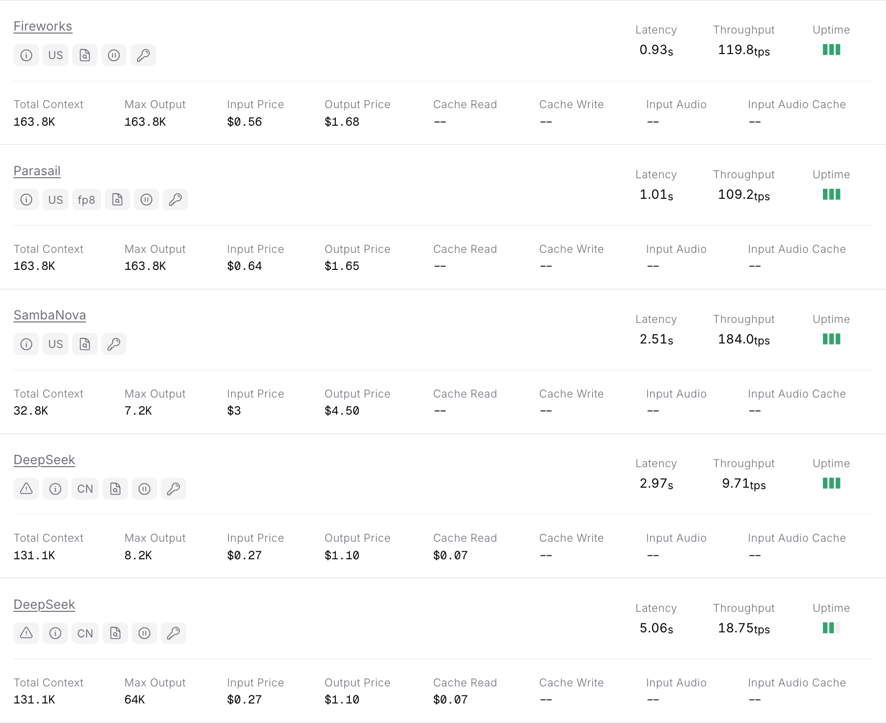
Due to "policy and regulatory constraints", aka export restrictions, the DeepSeek team is operating under severe compute constraints, both for training and for inference of their models. This hardware scarcity is evident when inspecting the average throughput of DeepSeek V3.1 reported by OpenRouter (see Fig. 10). While Western inference providers like Fireworks and Together serve it at a comfortable 60-80 tokens per second (tps), DeepSeek manages only ~25 tps.

For reasoning models, generating thousands of tokens before final answers, this leads to a significantly worse UX for interactive usecases. A typical math problem requiring 3,000 reasoning tokens takes 120 seconds (3000 tokens/ 25 tps) - forcing users into a 2-minute wait that limits practical applications to scenarios where user’s latency tolerance is high.

Faced with hardware scarcity, DeepSeek did what any good engineer would do: they got creative. Rather than designing for perfect conditions they'll never have, they optimized everything around their actual constraints. The inference optimizations detailed in a recent paper by DeepSeek - from expert routing to MLA-MoE computation overlap to networking topology - reflect this constraint-driven mindset. We examine several optimizations that most impact our theoretical cost model.

Figure 10: Average DeepSeek V3.1 throughput as measured by OpenRouter. Note how much slower than the Western providers DeepSeek is on average. This throughput difference suggests constrained hardware allocations, likely forcing DeepSeek to prioritize larger batch sizes over individual request latency. While this strategy reduces per-token serving costs through higher GPU utilization, it comes at the expense of user experience. 31.08.2025

Expert Parallelism

As shown later, expert layers contain approximately 661B parameters, representing 98.5% of the total parameter count. This distribution necessitates careful consideration of parallelization strategies. To minimize weight-related overhead, parameter distribution rather than duplication provides the optimal approach.

In traditional tensor parallel configurations with dense FFN layers, communication involves dispatching and combining hidden-size values per token and layer. MoE models introduce complexity because batch tokens route to different model components (different experts). Given the compact dimensions of expert weight matrices (d-moe=2048), tensor parallel sharding would fragment these matrices into excessively small components, resulting in suboptimal blocked matrix multiplication performance. Expert parallel sharding preserves matrix integrity, enabling more efficient memory access patterns during GEMM operations.

However, this approach increases total communication overhead to

\(d\times (n_r^E + n_s^E)\)

per token and layer, where d is the model's hidden size. Because experts may reside on different devices, expert parallel distribution becomes more exposed to communication bottlenecks, fundamentally changing the performance characteristics compared to dense models.

For deployments with small numbers of devices, particularly single or dual-node configurations, or those with very bad inter-node communication hardware, tensor parallel sharding can achieve superior performance due to the reduced communication overhead.

Expert Parallel Load Balancing

Expert routing probabilities exhibit non-uniform distributions (see Fig. 11), causing some experts to receive disproportionately higher request volume while other experts remain underutilized. Naive uniform expert distribution across available devices creates two critical performance issues: (1) uneven communication patterns where bottlenecks stall entire forward passes, and (2) asymmetric computational loads across devices. Additionally, heavily utilized devices must handle increased activation loading and memory write-back operations, compounding performance degradation.

Load balancing strategies can mitigate these issues through intelligent expert distribution across devices to achieve more uniform computational loads. Furthermore, frequently accessed experts can be duplicated to reduce communication peaks, though this approach carries the trade-off of increased weight loading and reduced per-GPU KV cache capacity. Since the expert layer computation is most often memory bound, having the same number of experts on each device is optimal. Therefore, the number of additional experts per layer must be constrained to multiples of the expert parallel size.

An interesting use case are uneven node configurations, where redundant experts can be used to fill up underutilized devices to achieve balanced expert distribution. For instance, the SGLang team reported using nine nodes for decode operations (72 expert parallel size) with 32 additional experts, achieving favorable trade-offs between additional memory overhead and reduced communication peaks.

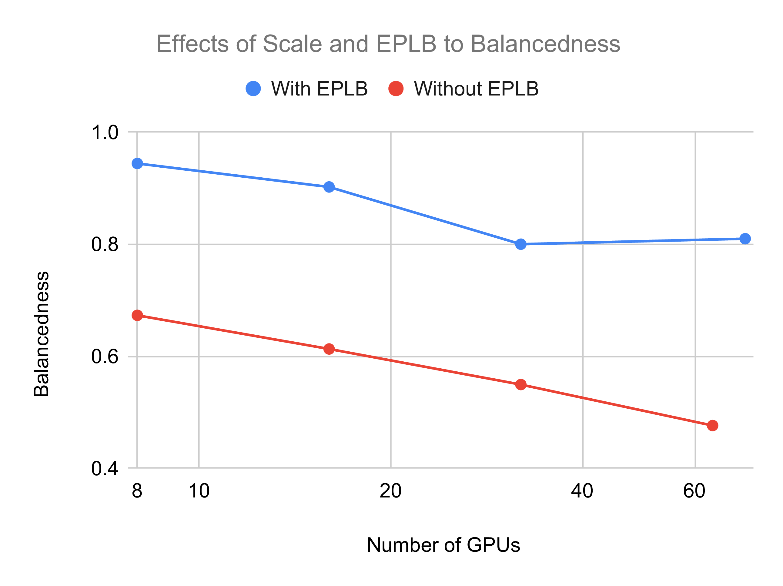
Importantly, expert load balancing becomes increasingly challenging as node count increases. This degradation occurs because fewer nodes concentrate more experts per device, increasing the probability of achieving system-wide balance. So for deployments on very few nodes, the improvement in expert balancedness is not worth the corresponding redundant experts.

Figure 11: Expert imbalance during prefill and decode phases as reported by SGLang. These are empirical observations from running over some specific datasets, so in your particular application the exact distribution will differ. The meta point, that experts usage is not uniformly distributed, stands, though.

Location-Aware Expert Selection

To minimize the limiting inter-node communication, expert selection can incorporate locality penalties that preferentially route tokens to experts residing on the same node where their attention computations were performed. This approach reduces cross-node communication overhead, which often represents a primary bottleneck in distributed MoE inference.

During training, DeepSeek V3 implemented expert routing constraints ensuring each token routes to at most M nodes. Node selection follows the sum of the highest Kᵣ/M affinity scores for experts distributed on each node, where Kᵣ represents the number of routed experts and M the maximum number of nodes per token.

This methodology can be adapted for inference scenarios but requires careful tuning to balance locality benefits against response quality. A notable consequence of this approach is that token routing patterns become dependent on the position of the sequence within the batch, potentially creating position-dependent expert utilization patterns that may affect model responses.

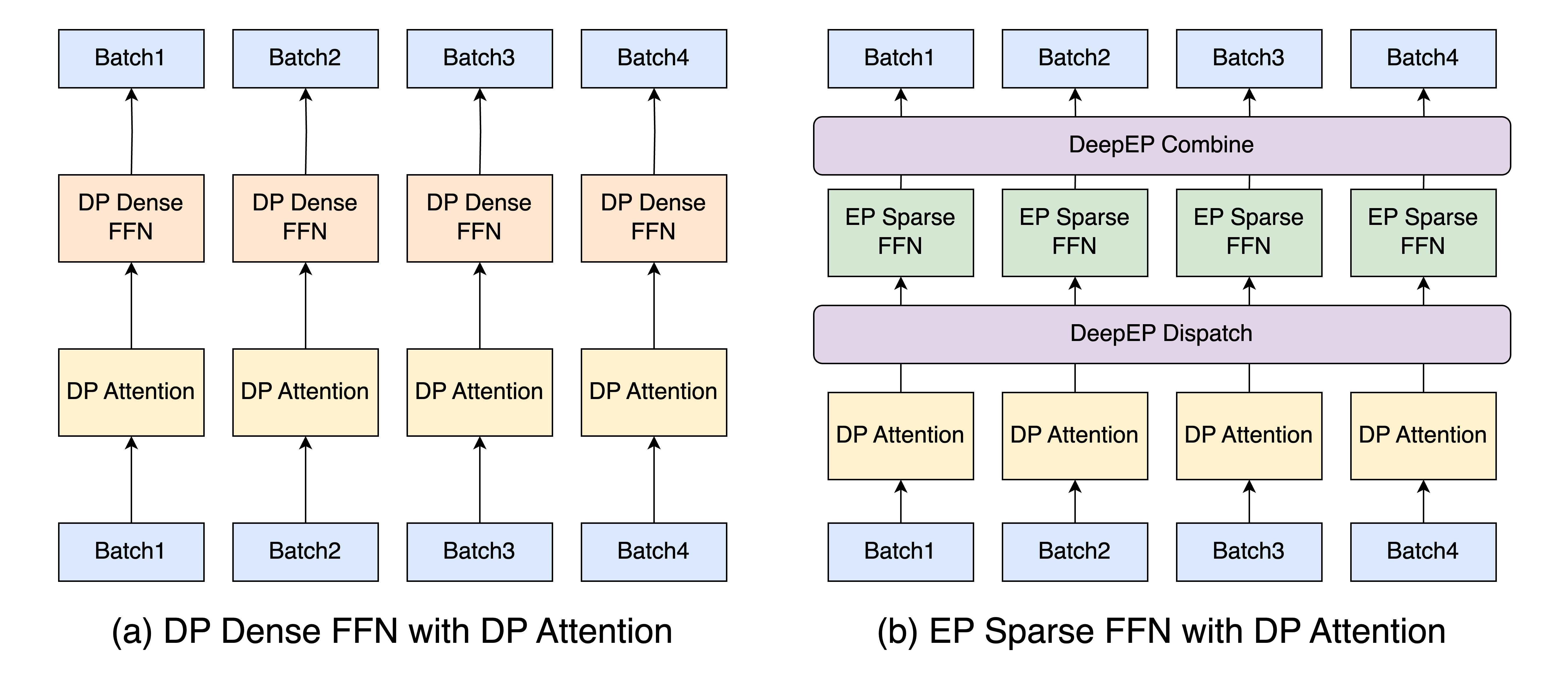
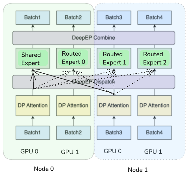
Data Parallel Attention

Attention computation employs a data-parallel approach, distributing requests across available devices (see Fig. 12). This strategy enables KV cache sequences to remain on single devices, eliminating the need for duplication or inter-device communication of the latent KV cache, which, on the other hand, would be required under tensor-parallel MLA computation due to projection matrices.

However, this data-parallel approach requires duplicating all MLA weights across devices, approximately 10 GB for DeepSeek V3.1, and they must be loaded during each forward pass. This presents scalability tradeoffs for large-scale deployments. Specifically, in configurations exceeding 64 GPUs, the MLA weight parameters can consume greater memory resources than the expert layers themselves. This duplication reduces available KV cache capacity and renders MLA computations memory-bound for most batch sizes.

Figure 12: Visualization of DP Attention from SGLang blogpost. Different GPUs process different microbatches. It works both for dense layers (first 3 layers in DeepSeek) and mixture-of-experts layers.

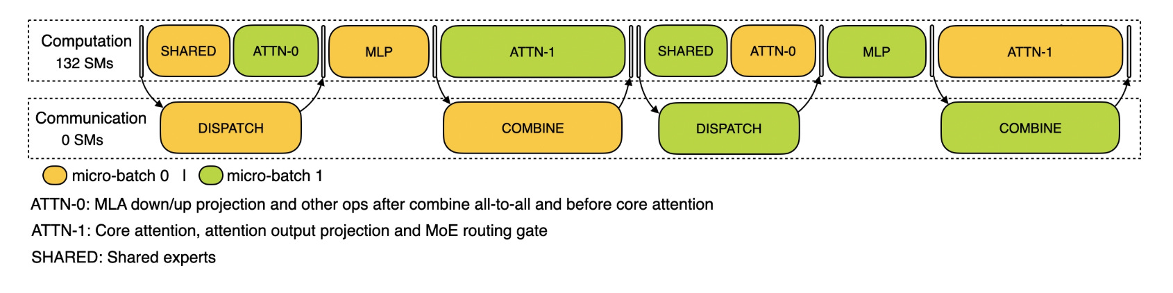
Hiding Communication with Two-Batch Overlap

As shown previously, expert parallelism in MoE models generates approximately nine times the communication volume compared to traditional tensor parallelism. To mitigate this overhead, a two-batch overlap (TBO) strategy can be implemented to mask communication time behind computation. This approach partitions the global batch size into two micro-batches, enabling simultaneous execution where one micro-batch performs computation while the other handles communication operations.

Effective overlap implementation requires careful orchestration of computational and communication phases. Figure 13 illustrates a basic TBO configuration for decode operations. Since communication operations consume minimal computational resources, TBO can achieve runtime improvements of close to a factor of two in certain scenarios.

Figure 13: Creating two mini-batches allows for overlapping the communication of one mini-batch with the computation of the other, thus in most cases hiding the communication from the overall runtime. Depending on the inference regime, different overlapping structures can be used. The figure depicts DeepSeeks setup for the decode phase during inference. Figure taken from DeepSeek's profiling of V3.

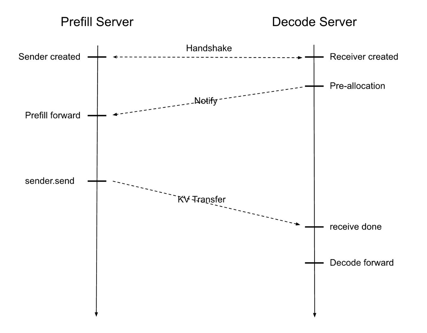
Prefill Decode Disaggregation

LLM inference comprises two distinct phases with fundamentally different computational characteristics. Prefill operations process entire input sequences simultaneously, creating compute-intensive workloads with high FLOP utilization but minimal KV cache requirements. Decode operations generate tokens iteratively, resulting in memory-bandwidth-bound computations. Also, decoding is much more latency sensitive due to its repetitive nature.

As explained in more detail on SGLang's blog post traditional unified engines process prefill and decode batches together, introducing three critical inefficiencies: (1) incoming prefill batches interrupt ongoing decode operations, causing substantial token generation delays; (2) data-parallel attention imbalances occur when workers simultaneously handle different batch types, increasing decode latency; and (3) incompatibility arises with advanced expert placement strategies that require different dispatch modes for each phase.

Prefill-decode disaggregation resolves these issues by separating workloads into dedicated clusters optimized for each phase's requirements, with prefill usually needing fewer resources than decode due to better compute utilization.

Figure 14: Upon receiving an input request, the workflow proceeds as follows: 1) A Prefill Server and a Decode Server pair via a handshake, establishing a local sender and receiver, respectively. 2) The Decode Server pre-allocates the KV cache, signaling the Prefill Server to begin the model forward pass and compute the KV caches. 3) Once computed, the data transfers to the Decode Server, which handles iterative token generation. As per SGLang blogpost.

Theoretical Performance Model

The theoretical performance model creates a virtual clone of our DeepSeek V3.1 model, enabling analysis of different hardware configurations to determine optimal MoE model serving strategies. Additionally, this framework allows identification of system bottlenecks across various deployment scenarios. While this model is specifically designed for DeepSeek V3 architecture, extensions to Kimi-K2 and other MoE architectures are quite simple.

The theoretical performance model analyzes attention (MLA in the case of DeepSeek V3.1) and expert computations separately, as these components may be constrained by different resources at different times. Since two-batch overlap techniques may be employed to hide communication, these two parts of the model may operate without overlap and are thus not able to hide the memory loading over both computations combined. Furthermore, the model accounts for communication across potentially heterogeneous networks incorporating different intra- and inter-node communication hardware. Communication time can be optionally overlapped using TBO. Finally, we consider scenarios where expert distribution is nonhomogeneous, resulting in imbalanced communication, increased memory loading, and uneven computation across GPUs, which can bottleneck the entire system.

With communication computation overlap, we define the total system performance as:

\(t_{total} = \max(t_{\text{bottleneck_MLA}} + t_{\text{bottleneck_EP}}, t_{\text{communication}})\)

Without TBO, we can (1) look at the memory loading time and compute time for each block (EP and attention) and take the maximum; (2) add the communication time; and (3) consider imbalanced experts:

\(t_{total} = t_{\text{bottleneck_MLA}} + t_{\text{bottleneck_EP}} + t_{\text{communication}}\)

The model operates under the following assumptions:

• No computational and memory loading overhead from the DeepEP TBO communication library. This assumption does not hold in practice, as the library launches a non-negligible number of CUDA kernels.

• All computations and weights are performed and stored in FP8, with the exception of communication operations, where dispatch occurs in BF16. This assumption is largely accurate since over 98% of parameters reside in expert weights, which utilize 8-bit quantization.

• The analysis focuses exclusively on decode performance without considering prefill operations. Theoretical derivations for prefill performance will be presented.

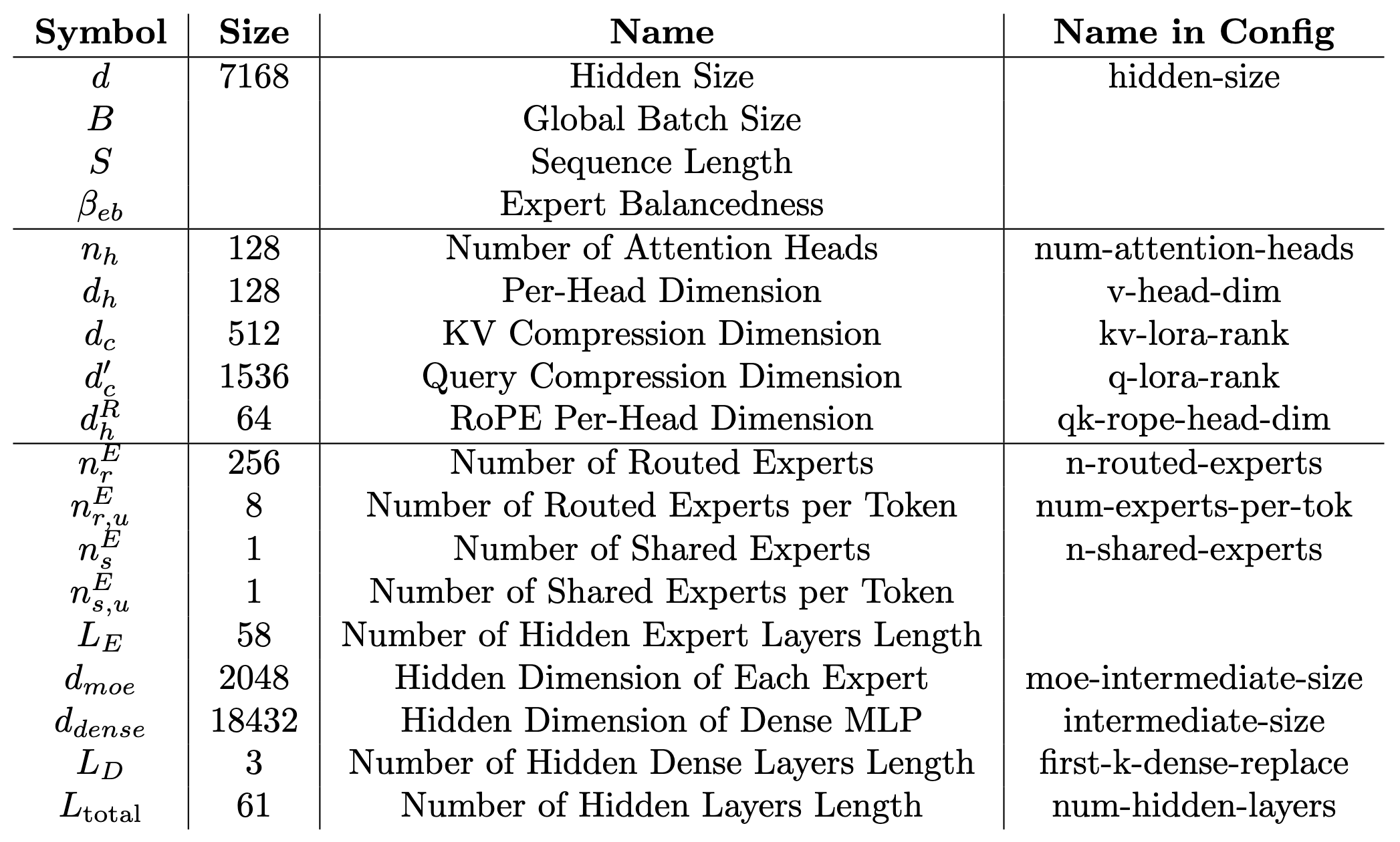
First lets look at the execution times of the MLA and expert MLP networks of a transformer block based on the operations performed and the memory loaded. Second we consider the communication. For reference all variable names are listed in Table 1.

Table 1: Nomenclature of the symbols used in this description for DeepSeek V3, including the name in the publicly available config.json file.

Memory Loading

To estimate the time spent loading from memory, we look at what gets loaded during each forward pass. First let's look at the MLA secondly at the expert networks.

MLA

The memory requirements during inference for the MLA can be categorized into three primary components: MLA weights (read), KV cache (read and write), and activations (write).

MLA weights are read once per forward pass. The MLA mechanism requires several weight matrices per layer, stored in FP8 format. As outlined for DeepSeek v2, during inference, the up-projection matrices for the K- and V-tensors can be included into other matrices, thus reducing the overall number of matrices.

\(W^{DQ} \in \mathbb{R}^{d_c' \times d} = 1536 \times 7168 = 11.0\text{MB}\)

\(W^{UQ} \in \mathbb{R}^{d_h \times n_h \times d_c'} = 128 \times 128 \times 1536 = 25.2\text{MB}\)

\(W^{QR} \in \mathbb{R}^{d^R_h \times n_h \times d_c'} = 64 \times 128 \times 1536 = 12.6\text{MB}\)

\(W^{DKV} \in \mathbb{R}^{d_c \times d} = 512 \times 7168 = 3.7\text{MB}\)

\(W^{UK} \in \mathbb{R}^{d_h \times n_h \times d_c} = 128 \times 128 \times 512 = 8.4\text{MB}\)

\(W^{UV} \in \mathbb{R}^{d_h \times n_h \times d_c} = 128 \times 128 \times 512 = 8.4\text{MB}\)

\(W^{KR} \in \mathbb{R}^{d^R_h \times d} = 64 \times 7168 = 0.5 \text{MB}\)

\(W^{O} \in \mathbb{R}^{d \times d_h \times n_h} = 7168 \times 128 \times 128 = 117.4\text{MB}\)

This yields a total of 187.2 MB per layer, resulting in 11.4 GB total attention weights that must be replicated across each data-parallel attention rank.

KV Cache size is significantly reduced in MLA architectures compared to traditional attention mechanisms. The cache size per token is determined by

\((d_c + d_R^h)\times L\)

where d_c = 512 represents the KV compression dimension, d^h_R = 64 denotes the per-head dimension of decoupled queries and keys, and L = 61 is the number of layers.

The memory requirement becomes:

\(2 \times (d_c + d_R^h) \times L = 2 \times (512 + 64) \times 61 = 70\text{KB per token}\)

For a batch processing S input tokens and generating B output tokens, the system loads S x B tokens and saves B tokens to cache.

Activation vectors require temporary storage for communication between expert computations. These activations are loaded once and written back once during the forward pass:

\(A = 2 \times B \times d \times L \approx B \times 0.9\text{MB}\)

While non-negligible for very large batch sizes, activation memory remains relatively small compared to weight and cache requirements.

Expert Networks

For the expert MLP networks, we have two sources of memory transfers: model weights, which get read once for each forward pass; and activations, which get loaded once in FP8 and written back once in BF16.

The latent vectors are loaded from and saved back to memory for communication. We load them once in FP8 and write them back once in BF16. This part is often negligible.

\(\begin{aligned}A&=(1+2)\times B\times d \times L \approx B\times 1.4 MB\\ A_\text{total per GPU}&=(1+2)\times B\times d \times L \times \frac{1}{\beta_{eb}} \times \frac{n_{\text{shared_experts_used}} + n_{\text{routed_experts_used}}}{n\_GPUs}\end{aligned}\)

The expert MLP is made up of two weight matrices W_1 and W_2, which perform a down-projection followed by an up-projection. Note that traditional transformer models have a larger intermediate space thus they first up-project, which makes the matrices much larger. Secondly, we have to account for the SwiGLU gate weight matrix as well. So the size of one expert is

\(\begin{aligned}W_1=W_2&= d_{moe} \times d = 2048 \times 7168 \approx 14.7 \text{MB}\\ W_{\text{Gate}} &= d_{moe} \times d = 2048 \times 7168 \approx 14.7 \text{MB}\\ W_E &= W_1 + W_\text{Gate}+ W_2 = 3\times \text{moe_intermediate_size} \times d \approx 45\text{MB}.\end{aligned}\)

Lastly, we have to account for the router in each expert which is of size

\(W_{\text{router}} = d \times \text{routed_experts}\)

To get the expert weights per devices, the weights are distributed evenly over the devices. Additionally we assume that one device has to hold the full router (overestimation). So for each expert layer we get:

\(\begin{aligned}&W_{\text{experts per GPU}} = n_{\text{layers}}^\text{experts}\times \\ &\left( W_E \times \lceil \frac{n_{\text{shared_experts}} + n_{\text{routed_experts}} + n_{\text{additional_experts}}}{n\_GPUs} \rceil + W_{\text{router}}\right)\end{aligned}\)

For DeepSeek V3.1 not all transformer layers are using the MoE architecture. The first three layers are made from traditional dense MLPs. Using d_dense as the intermediate size we get:

\(\begin{aligned}W_1^d=W_2^d&= d_{dense} \times d = 18432 \times 7168 \approx 132 \text{MB}\\ W_{\text{Gate}}^d &= d_{dense} \times d = 18432 \times 7168 \approx 132 \text{MB}\\ W_{MLP}^d &= W_1^d + W_\text{Gate}^d+ W_2^d = 3\times d_{dense} \times d \approx 396\text{MB}.\end{aligned}\)

When serving in expert parallel with SGLang these weights are sharded data parallel. Thus:

\(W_{\text{MLP per GPU}}^\text{dense} = n_{\text{layers}}^\text{dense}\times W_{MLP}^d\approx 3 \times 396\text{MB} \approx 1.2\text{GB}\)

Embedding Layers

The embedding matrix size is V x d, where V is the vocabulary size. As we need to embed and un-embed, and each embedding matrix is sharded across GPUs in a data-parallel fashion, the per-GPU size is:

\(W_{\text{E per GPU}} = 2\times V\times d = 2 \times 129280\times 7168 \approx 1.9 \text{GB}\)

As this is a large matrix with V » 100k, we assume this calculation is always memory-bound, and thus we only take into account the memory loading time.

Computation

To quantify computational latency, we examine the multi-head latent attention (MLA) mechanism following the architectural specification detailed in DeepSeek v2 Appendix C. Our analysis incorporates matrix absorption optimizations that enable certain linear transformations to be merged during inference. We validate our computational framework against the DeepSeek V3 training time calculator to ensure consistency, though we need to employ some changes due to optimizations only possible during inference. Furthermore, the single-token generation characteristic of decode operations substantially simplifies several equations relative to training contexts where full sequence processing is required. We denote computations specific to prefill scenarios with Prefill annotations to distinguish where prefill diverges from decode execution paths.

Our computational analysis has three main parts: a vanilla MLA implementation baseline, optimized MLA with matrix absorption techniques, and expert network computational latency.

MLA

MLA computational demands differ substantially between prefill and decode phases due to sequence length scaling characteristics, necessitating phase-specific analysis of each MLA component. We begin by reviewing the MLA computation procedure as specified in DeepSeek v2 Appendix C:

\(\begin{align*} \mathbf{c}_t^Q &= W^{DQ} \mathbf{h}_t, \\ \left[ \mathbf{q}_{t,1}^C; \mathbf{q}_{t,2}^C; \dots; \mathbf{q}_{t,n_h}^C \right] &= \mathbf{q}_t^C = W^{UQ} \mathbf{c}_t^Q, \\ \left[ \mathbf{q}_{t,1}^R; \mathbf{q}_{t,2}^R; \dots; \mathbf{q}_{t,n_h}^R \right] &= \mathbf{q}_t^R = \text{RoPE}(W^{QR} \mathbf{c}_t^Q), \\ \mathbf{q}_{t,i} &= \left[ \mathbf{q}_{t,i}^C; \mathbf{q}_{t,i}^R \right], \\ \mathbf{c}_t^{KV} &= W^{DKV} \mathbf{h}_t, \\ \left[ \mathbf{k}_{t,1}^C; \mathbf{k}_{t,2}^C; \dots; \mathbf{k}_{t,n_h}^C \right] &= \mathbf{k}_t^C = W^{UK} \mathbf{c}_t^{KV}, \\ \mathbf{k}_t^R &= \text{RoPE}(W^{KR} \mathbf{h}_t), \\ \mathbf{k}_{t,i} &= \left[ \mathbf{k}_{t,i}^C; \mathbf{k}_{t,i}^R \right], \\ \left[ \mathbf{v}_{t,1}^C; \mathbf{v}_{t,2}^C; \dots; \mathbf{v}_{t,n_h}^C \right] &= \mathbf{v}_t^C = W^{UV} \mathbf{c}_t^{KV}, \\ \end{align*}\)

\(\begin{align*} \mathbf{o}_{t,i} &= \sum_{j=1}^t \text{Softmax}_j \left( \frac{\mathbf{q}_{t,i}^T \mathbf{k}_{j,i}}{\sqrt{d_h + d_h^R}} \right) \mathbf{v}_{j,i}^C, \\ \mathbf{u}_t &= W^O \left[ \mathbf{o}_{t,1}; \mathbf{o}_{t,2}; \dots; \mathbf{o}_{t,n_h} \right], \end{align*}\)

where c_t^Q, c_t^{KV} are the compressed Q and KV tensors respectively. During decode operations, MLA requires up-projecting the K- and V-tensors for every token within the cache, leading to significant computational overhead. To mitigate this burden, the up-projection matrices for K- and V-tensors can be absorbed into existing matrix operations, thereby reducing the total number of matrix-vector multiplications, as briefly touched upon in the DeepSeek v2. Through computational reordering, the self-attention mechanism, for instance, transforms to:

\(\begin{aligned} q_{t,i}^T k_{j,i} &= (W^{UQ}_{[i \times n_h:(i+1), :]} c^Q_t)^T W^{UK}_{[i \times n_h:(i+1), :]} c^{KV}_j + q_{t,i}^{R^T} k_{j,i}^R \\ &= c^{QT}_t (W^{{UQ}^T} W^{UK})_{[i \times n_h:(i+1), :]} c^{KV}_{j,i} + q_t^{R^T} k_{j,i}^R, \end{aligned}\)

The most important advantage, as demonstrated in the following sections, is that the KV cache no longer requires up-projection operations. We apply analogous reordering to the V-tensor up-projection weight matrix W^{UV}, absorbing it into the output projection matrix W^O.

However, materializing

\(W^{{UQ}^T} W^{UK}\)

increases the amount of memory transfer and reduces available KV cache capacity. But there is a way to have our cake and eat it. Our approach diverges from DeepSeek's hint by avoiding materialization of the resulting composite matrix. Instead, we achieve efficiency through dynamic computation: rather than storing the composite matrix

\(W^{{UQ}^T} W^{UK}\)

we compute it on-demand during each forward pass while calculating q_t^C. This strategy maintains an identical memory footprint and loading patterns while eliminating the computationally expensive sequence-length dependency imposed upon us due to the up-projections of K- and V-tensors during the decode phase.

To understand the computational requirements of MLA, we begin with analyzing the straightforward vanilla implementation to establish baseline FLOP counts, then progress to the optimized variant and show its performance improvements.

Vanilla MLA Implementation

The vanilla implementation follows the MLA specification from DeepSeek v2 Appendix C, comprising three phases: latent projection, self-attention, and output projection.

Latent Up-/Down-Projection The latent projection involves two sequential operations: down-projection to the latent space, followed by up-projection to the attention dimension. For the sake of simplicity, we ignore the RoPE and Softmax calculations.

Prefill:

\(\begin{align} \style{color:grey}{FLOPs_\text{q_down_proj}} &\style{color:grey}{= 2 \times B \times S \times d \times d_c'} \\ \style{color:grey}{FLOPs_\text{q_up_proj}} &\style{color:grey}{= 2 \times B \times S \times d_c' \times n_h \times d_h} \\ \style{color:grey}{FLOPs_\text{q_RoPE_proj}} &\style{color:grey}{= 2 \times B \times S \times d_c' \times n_h \times d^R_h} \\ \style{color:grey}{FLOPs_\text{kv_down_proj}} &\style{color:grey}{= 2 \times B \times S \times d \times d_c} \\ \style{color:grey}{FLOPs_\text{k_up_proj}} &\style{color:grey}{= 2 \times B \times S \times n_h \times d_c \times d_h^{qk}} \\ \style{color:grey}{FLOPs_\text{k_RoPE_proj}} &\style{color:grey}{= 2 \times B \times S \times d \times d^R_h} \\ \style{color:grey}{FLOPs_\text{v_up_proj}} &\style{color:grey}{= 2 \times B \times S \times n_h \times d_c \times d_h^{v}} \end{align}\)

During decode operations, most sequence-length dependencies can be eliminated since intermediate values are either used once or cached. However, performing K- and V-tensor projections for each token in the context remains necessary due to caching in latent format. This creates a problematic sequence-length dependency that significantly degrades performance. So vanilla decode projection becomes Decode (single token):

\(\begin{align} FLOPs_{\text{q_down_proj}} = 2 \times B \times d \times d_c' \\ FLOPs_{\text{q_up_proj}} = 2 \times B \times d_c' \times n_h \times d_h \\ FLOPs_{\text{q_RoPE_proj}} = 2 \times B \times d_c' \times n_h \times d^R_h \\ FLOPs_{\text{kv_down_proj}} = 2 \times B \times d \times d_c \\ FLOPs_{\text{k_up_proj}} = 2 \times B \times S \times n_h \times d_c \times d_h^{qk} \\ FLOPs_{\text{k_RoPE_proj}} = 2 \times B \times d \times d^R_h \\ FLOPs_{\text{v_up_proj}} = 2 \times B \times S \times n_h \times d_c \times d_h^{v} \end{align}\)

where the FLOPs_{k_RoPE_proj} only need to be calculated once for each k, as they are cached.

Attention Computation The attention mechanism computes query-key interactions against cached key-value pairs, exhibiting computational complexity that scales with sequence length.

Prefill:

\(\begin{align} \style{color:grey}{FLOPs_\text{qk_scores}} &\style{color:grey}{= 2 \times B \times S^2 \times n_h \times (d_h + d^R_h)} \\ \style{color:grey}{FLOPs_\text{$\times$v}} &\style{color:grey}{= B \times S^2 \times n_h \times d_h} \end{align}\)

Decode:

\(\begin{align} FLOPs_\text{qkv} &= B \times n_h \times S \times (2 \times (d_h + d^R_h) + d_h) \end{align}\)

Output Linear Transformation The final linear transformation projects attention outputs back to the model's hidden dimension:

Prefill:

\(\begin{equation} \style{color:grey}{FLOPs_\text{out_lin} = 2 \times B \times S \times n_h \times d_h \times d} \end{equation}\)

Decode:

\(\begin{equation} FLOPs_\text{out_lin} = 2 \times B \times n_h \times d_h \times d \end{equation}\)

We now examine the computational modifications when implementing the non-materialized matrix-absorption approach.

Matrix-Absorbed MLA Implementation

The primary goal of the two matrix absorptions:

\(W^{UK} \to W^{UQ} \text{ and } W^{UV} \to W^{O}\)

is to eliminate per-token KV cache up-projections by enabling direct computation on compressed KV-tensors. This fundamentally alters the memory access pattern.

Latent Up-/Down-Projection Since we absorb the up-projection matrices for K- and V-tensors, we no longer need to perform these projections.

Prefill:

\(\begin{align} \style{color:grey}{FLOPs_\text{q_down_proj}} &\style{color:grey}{= 2 \times B \times S \times d \times d_c'} \\ \style{color:grey}{FLOPs_\text{q_RoPE_proj}} &\style{color:grey}{= 2 \times B \times S \times d_c' \times n_h \times d^R_h} \\ \style{color:grey}{FLOPs_\text{kv_down_proj}} &\style{color:grey}{= 2 \times B \times S \times d \times d_c} \\ \style{color:grey}{FLOPs_\text{k_RoPE_proj}} &\style{color:grey}{= 2 \times B \times S \times d \times d^R_h} \\ \end{align}\)

Decode:

\(\begin{align} FLOPs_\text{q_down_proj} &= 2 \times B \times d \times d_c' \\ FLOPs_\text{q_RoPE_proj} &= 2 \times B \times d_c' \times n_h \times d^R_h\\ FLOPs_\text{kv_down_proj} &= 2 \times B \times d \times d_c \\ FLOPs_\text{k_RoPE_proj} &= 2 \times B \times d \times d^R_h, \end{align}\)

This eliminates the sequence-length dependency during the projection stage, which constitutes a significant computational bottleneck.

Attention Computation In this self-attention computation, we need to take the absorbed

\(W^{{UQ}^T} W^{UK}\)

into account.

Prefill:

\(\begin{align} \style{color:grey}{FLOPs_\text{q $W^{UQ^T}$}} &\style{color:grey}{= 2 \times B \times S \times n_h \times d_h \times d_c'} \\ \style{color:grey}{FLOPs_\text{$\times W^{UK}$}} &\style{color:grey}{= 2 \times B \times S \times n_h \times d_h \times d_c} \\ \style{color:grey}{FLOPs_\text{qk_scores}} &\style{color:grey}{= 2 \times B \times S^2 \times n_h \times (d_c + d_h^R)} \\ \style{color:grey}{FLOPs_\text{$\times$v}} &\style{color:grey}{= B \times S^2 \times n_h \times d_c} \end{align}\)

Decode:

\(\begin{align} FLOPs_\text{q $W^{UQ^T}$} &= 2 \times B \times n_h \times d_h \times d_c' \\ FLOPs_\text{$\times W^{UK}$} &= 2 \times B \times n_h \times d_h \times d_c \\ FLOPs_\text{qk_scores} &= 2 \times B \times S \times n_h \times (d_c + d_h^R) \\ FLOPs_\text{$\times$v} &= B \times S \times n_h \times d_c, \end{align}\)

As shown, the sequence-length dependency is eliminated for FLOPs×W^(UK) and FLOPs×W^(UV) without introducing additional matrix materialization.

Output Linear Transformation The final linear transformation again projects attention outputs to the model dimension, incorporating the absorption of W^UV into W^O. We again avoid materializing the absorbed matrix to minimize memory overhead.

Prefill:

\(\begin{equation} {FLOPs_\text{out_lin} = 2 \times B \times S \times (n_h \times d_h \times d + n_h \times d_h \times d_c)} \end{equation}\)

Decode:

\(\begin{equation} FLOPs_\text{out_lin} = 2 \times B \times (n_h \times d_h \times d + n_h \times d_h \times d_c) \end{equation}\)

Expert Networks

Following the MLA computational analysis, expert-network computation is relatively simple. Each expert module comprises two components: (1) a router and (2) the experts themselves. The experts consist of two layers with inverse dimensions and a SwiGLU activation function, incorporating gate projection weights of matching dimensions.

\(\begin{align} \text{Down-projection: } & B \times 2 \times d \times d_\text{moe} \\ \text{Up-projection: } &B \times 2 \times d \times d_\text{moe} \\ \text{Gate projection: } &B \times 2 \times d \times d_\text{moe} \\ \end{align}\)

In total, for all experts, we get:

\(\begin{align} FLOPs_{\text{linear_layers}}&=3\times 2 \times B \times d \times d_{\text{moe}}\\ FLOPs_{\text{router}}&=2 \times B \times d \times n_r^E \\ FLOPs_{\text{moe_total}}&=FLOPs_{\text{linear_layers}} \times (n_s^E + n_{r,u}^E) + FLOPs_{\text{router}}. \end{align}\)

With expert imbalance (characterized by the expert imbalance factor β_eb that we introduce in later sections),

\($FLOPs_{\text{moe_total}}= FLOPs_{\text{linear_layers}} \times \frac{1}{\beta_{eb}} \times \frac{n_{s,u}^E + n_{r,u}^E}{n_GPUs} + \frac{FLOPs_{\text{router}}}{n_GPUs}$\)

Communication

Communication Base Model

Following the analysis presented in the SGLang blog post, the only inter-GPU communications stem from expert-parallelism sharding. Figure 16 illustrates this communication pattern during forward passes within individual layers. Each layer has two distinct communication phases: a dispatch phase routing tokens from data-parallel MLA blocks to selected experts, followed by a combine phase aggregating expert computation results for propagation to the next data-parallel MLA block in the subsequent layer.

Figure 16: Communication pattern during expert-parallel sharding. Each GPU sends out n(r,u)^E + n(s,u)^E = 9 messages going from the MLA to the expert computation and receives n(r,u)^E + n(s,u)^E = 9 many messages going from the experts computation to the next MLA step. This communication can happen intra- or inter-node, where systems with larger EP size increase the percentage of inter-node communication. The base image was taken from the SGLang blog post.

The DeepSeekV3 scaling analysis establishes a baseline communication model assuming uniform expert distribution across devices, where "each device holds one expert’s parameters and processes approximately 32 tokens at a time". This configuration corresponds to a 257-GPU deployment with homogeneous network connections (each GPU-to-GPU connection has the same bandwidth and latency). We extend their formulation to accommodate arbitrary system configurations under assumptions of uniform network topology and perfectly balanced expert allocation. For each GPU communication link, each dispatch and combine operation processes

\(\frac{B}{2\times n_{\text{GPUs}}}\)

tokens (accounting for dual-batch overlap), with replication across

\(n_{total,u}^E = n_{r,u}^E + n_{s,u}^E$\)

The total communication volume per GPU link per forward pass for DeepSeek V3.1 architectures becomes:

\(\begin{aligned} \text{comm_amount}_{\text{v3 / r1}} &= \underbrace{2}_{\substack{\text{2b-overlap} \\ \text{$\rightarrow$ 2 } \times \text{total time}}} \times \underbrace{(1\text{Byte} + 2\text{Bytes})}_{\substack{\text{dispatch in FP8 (1 byte),} \\ \text{combine in BF16 (2 bytes)}}} \times \frac{B}{2 \times n_{\text{GPUs}}} \times n_{total,u}^E \times d \times L \\ & = 2 \times \frac{B}{2 \times n_{\text{GPUs}}} \times 3 \times (8+1) \times 7168 \times 61 \\ &= \frac{B}{n_{\text{GPUs}}} \times 0.0118 \text{ GB}. \end{aligned}\)

The leading factor of 2 reflects computation-communication micro-batch overlap, where consecutive batch processing introduces sequential dependencies. Dispatch operations utilize FP8 precision while combine phases use BF16 precision.

The effective communication bandwidth corresponds to the minimum link bandwidth within the system topology. In well-balanced configurations without bottlenecks this is the link to each GPU. In general cases the constraint becomes:

\(\text{comm_bandwidth} = \min(\text{comm_bandwidth}_{\text{GPU}}, \frac{\text{comm_bandwidth}_{\text{system bottleneck}}}{n_{\text{GPUs using bottleneck}}}).\)

Within homogeneous network environments, the communication execution time follows:

\(t_{\text{comm}} = \text{comm_amount}_{\text{v3 / r1}} \times \frac{1}{\text{comm_bandwidth}}.\)

Improvement 1: Non-Heterogeneous Communication Links

Standard systems often have different interconnect speeds for intra- and inter-node communication. Given that 1/n_nodes of total communication volume remains within individual nodes, this fraction of communication becomes negligible in heterogeneous network configurations where interconnect speeds differ substantially (for example, NVLink at 450 GB/s versus InfiniBand at 50 GB/s). The NVL72 rack configuration represents a notable exception, providing uniform NVLink connectivity across all nodes within the rack.

For systems with heterogeneous interconnections, the total communication time becomes:

\(\begin{aligned} t_{\text{comm}} = \text{comm_amount}_{\text{v3 / r1}} \times max(& \frac{n_{\text{nodes}}-1}{n_{\text{nodes}}} \times \frac{1}{\text{comm_bandwidth}_{\text{inter-node}}}, \\ & \frac{1}{n_{\text{nodes}}} \times \frac{1}{\text{comm_bandwidth}_{\text{intra-node}}} ) \end{aligned}\)

Improvement 2: Expert Imbalance

Our initial analysis assumed uniform expert distribution across GPUs, enabling straightforward communication volume calculations from the data-parallel MLA perspective. However, this assumption breaks down in practical deployments. As an easy counter example, consider a system deploying 9 experts across 8 GPUs: one GPU must accommodate 2 experts due to the discreteness of the experts, resulting in nearly double the communication overhead compared to balanced configurations:

\(\begin{aligned} 2\times \underbrace{2}_{\substack{\text{2b-overlap} \\ \text{$\rightarrow$ 2 } \times \text{total time}}} \times \underbrace{(1\text{Byte} + 2\text{Bytes})}_{\substack{\text{dispatch in FP8 (1 byte),} \\ \text{combine in BF16 (2 bytes)}}} \times \frac{B}{2} \times d \times L &= 2\times B \times \frac{1}{8+1} \times 0.0118 \text{ GB} \\ & > \frac{B}{8} \times 0.0118 \text{ GB} \end{aligned}\)

While sufficiently large batch sizes with random expert routing (and appropriate shared expert replication) could theoretically rebalance this load, empirical measurements in production systems show inherent differences in expert utilization that contradicts this assumption.

From the perspective of individual GPUs hosting experts, the communication volume becomes:

\(\begin{aligned} \underbrace{2}_{\substack{\text{2b-overlap} \\ \text{$\rightarrow$ 2 } \times \text{total time}}} \times \underbrace{(1\text{Byte} + 2\text{Bytes})}_{\substack{\text{dispatch in FP8 (1 byte),} \\ \text{combine in BF16 (2 bytes)}}} \times \frac{B}{2} \times d \times L \times \frac{n_{total,u}^E}{n_{\text{GPUs}}}\\ \end{aligned}\)

Incorporating the expert load imbalance factor (introduced in the next section) into the formulation yields:

\(\text{comm_amount}_{\text{v3 / r1}} = B \times (1+2) \times d \times L \times \frac{1}{\beta_{eb}} \times \frac{n_{total,u}^E}{n_{\text{GPUs}}}\)

For heterogeneous network configurations, the resulting communication time then becomes:

\(\begin{aligned} t_{\text{comm}} &= \text{comm_amount}_{\text{v3 / r1}} \times \max\left( \frac{n_{\text{nodes}}-1}{n_{\text{nodes}}} \times \frac{1}{\text{comm_bandwidth}_{\text{inter-node}}}, \right.\\ &\left. \frac{1}{n_{\text{nodes}}} \times \frac{1}{\text{comm_bandwidth}_{\text{intra-node}}} \right) \end{aligned}\)

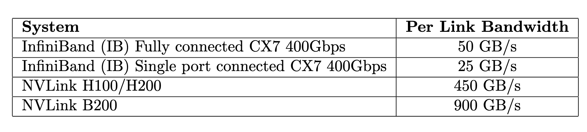
List of Common Interconnects

Table 2 presents unidirectional bandwidth specifications for all-to-all communication patterns for commonly used interconnect technologies, where communication throughput is constrained by the bandwidth available to individual GPUs (unidirectional bandwidth):

Table 2: Unidirectional bandwidth specifications across different interconnect technologies.

Expert Balancedness

The distribution of the experts over the GPUs can have a big impact on the communication and execution times of the expert layers. As an illustrative example, we can take a system with 2x8 H100 GPUs and distribute all the experts uniformly. In this case, there is a GPU which has the shared expert plus roughly 16 routed ones. Since all items in a batch will go to the shared expert, this GPU has to load roughly

\(\frac{1+\frac{n_{\text{shared_experts_used}} + n_{\text{routed_experts_used}}}{n_\text{GPUs}}}{\frac{n_{\text{shared_experts_used}} + n_{\text{routed_experts_used}}}{n_\text{GPUs}}} \approx 2,7\times\)

more activations than the other GPUs. Furthermore, 2.7 times more communication volume will go through the link connecting to the GPU.

To model this imbalance, we define and expose the variable β_eb to the user. Similar to the definition of SGLang, β_eb is defined as the ratio between mean expert load and maximum expert load among GPUs, so:

\(\beta_{eb} = mean_{layers}\left(\frac{\text{avg routed request per layer}}{\text{max routed request (of any GPU) per layer}}\right)\)

Therefore, β_eb_gpu=1 is a balanced case and β_eb=1/n_GPUs would be completely imbalanced. Thus the average load increases by L_imbalanced = (1/β_ep) × L_balanced.

For balancing the experts, some n_additional_experts get duplicated onto multiple GPUs. This can lead to an increase in EP memory loading time. As EP is often memory-bound, this can lead to an increased EP execution time. Thus balancing the experts is a tradeoff between loading more weights and more homogeneous communication and computation. Finally, one has to ensure that (n_routed_experts + n_additional_experts) modulo ep_size = 0, as otherwise imbalance in the memory loading and computations would be introduced by design.

Figure 17 from the SGLang blog post shows examples of expert balancedness given a number of GPUs and potentially active load balancing.

Figure 17: Achieved expert balancedness given a fixed number of devices using expert parallel load balancing. Source

From Parts to the Whole

Given all of these considerations, we implemented a theoretical model estimating the model throughput given the hardware. It should make it easier to understand the tradeoffs between the latency, throughput, and cost between different hardware providers.

The model includes a number of assumptions, such as:

• All weights are stored in FP8; the MLA is computed in BF16; the matrix multiplications in the expert layers are performed in FP8. The communication is done in FP8 apart from the dispatch which is done in BF16.

• We make some strong assumptions about the overhead for compute, memory bandwidth, and communication. We assume the same level of inefficiency across different hardware to make it fair. The levels are arbitrary and arguably can be one of the leading sources of error in our calculation. These inefficiencies in reality are also not the same for every hardware and are strongly dependent on the implementation.

• To make the calculations simpler we assume that no MTP is performed. We managed to make it run with MTP; however, we deemed the performance gains not worth the increase in complexity of the model, especially for larger batches.

• We only looked at the decode performance without taking into account prefill.

• We assume no compute and memory loading overheads from the DeepEP two-batch communication library. This is not true, as these operations start a significant number of CUDA kernels, which can have downstream effects on highly optimized kernels like GEMM, as they will no longer get the expected number of threads.

At a high level, the performance model comprises three primary execution components: MLA computation, expert parallel (EP) computation, and communication overhead. For both MLA and EP operations, we determine whether memory bandwidth or computational throughput constitutes the limiting factor. Communication can be optionally overlapped using two-batch overlap (TBO), where total execution time for one forward pass becomes

\(T_{TBO}=2\times T(B/2)\)

The high-level model structure follows:

\(\begin{align} T_{bottleneck}^{MLA}(B, S) &= \max\left(T_{mem}^{MLA}(B, S), T_{comp}^{MLA}(B, S)\right) \\ T_{bottleneck}^{EP}(B, S) &= \max\left(T_{mem}^{EP}(B, S), T_{comp}^{EP}(B, S)\right) \\ T_{total}^{\text{no }TBO} (B, S) &= T_{bottleneck}^{MLA}(B, S) + T_{bottleneck}^{EP}(B, S) + T_{comms}(B) \\ T_{total}^{TBO} (B, S) &= 2\times\max\left(T_{bottleneck}^{MLA}\left(\frac{B}{2}, S\right) + T_{bottleneck}^{EP}\left(\frac{B}{2}, S \right), T_{comms}\left(\frac{B}{2}\right)\right) \end{align}\)

Computational, memory, and communication time estimates use the previously derived formulae, adjusted for real-world implementation inefficiencies. Practical systems rarely achieve theoretical peak performance, necessitating inefficiency factors across all components. The DeepEP communication library documentation indicates 40 GB/s achieved throughput from 50 GB/s theoretical peak, yielding a communication overhead of ~25%. FlashMLA achieves approximately 66% MFU. Expert-layer computational performance, based on DeepGEMM benchmarks showing 1550 TFLOPs from 1980 TFLOPs theoretical FP8 dense peak performance results in an EP computation overhead factor of ~30%. Both computational inefficiencies receive an additional 10% penalty to account for suboptimal input conditions and overhead between the kernels.

Memory inefficiency estimation proves more challenging without profiling. Due to some operations, such as matrix multiplication, requiring multiple loading operations for the same value, and the fact that most kernels are optimized for compute bound scenarios, we apply a conservative inefficiency factor of 2.0 to account for these overheads.

Token generation rates are calculated as the inverse of total execution time, with global throughput scaling by concurrent batch size:

\(\begin{align} TPS_{request} &= \frac{1}{T_{total}^{TBO}} \\ TPS_{global} &= \frac{1}{T_{total}^{TBO}} \times B \end{align}\)

It is important to note that this model does not consider whether the proposed configurations are viable under real-world memory constraints. For instance, long context sequences can drastically reduce the maximum number of concurrent sequences due to memory limitations, resulting in significantly lower throughput than theoretical predictions.

Predictions and Real-World Comparison

To validate our theoretical model we compare it to real world measurements using three vastly different hardware setups:

• 4x8 H100: This is the basic setup that we consider reasonable to maintain by a large enterprise. This was also the setup we managed to obtain, therefore we have the measurements for all reasonable batch sizes.

• 9x8 H100: This is the setup from the SGLang blog post including their tuned performance measurements.

• 12x4 B200: This involves 48 out of 72 GPUs in an NVL72 setup. We use this to visualize how differently the new generation of hardware performs. This is also a setup tested by the SGLang team.

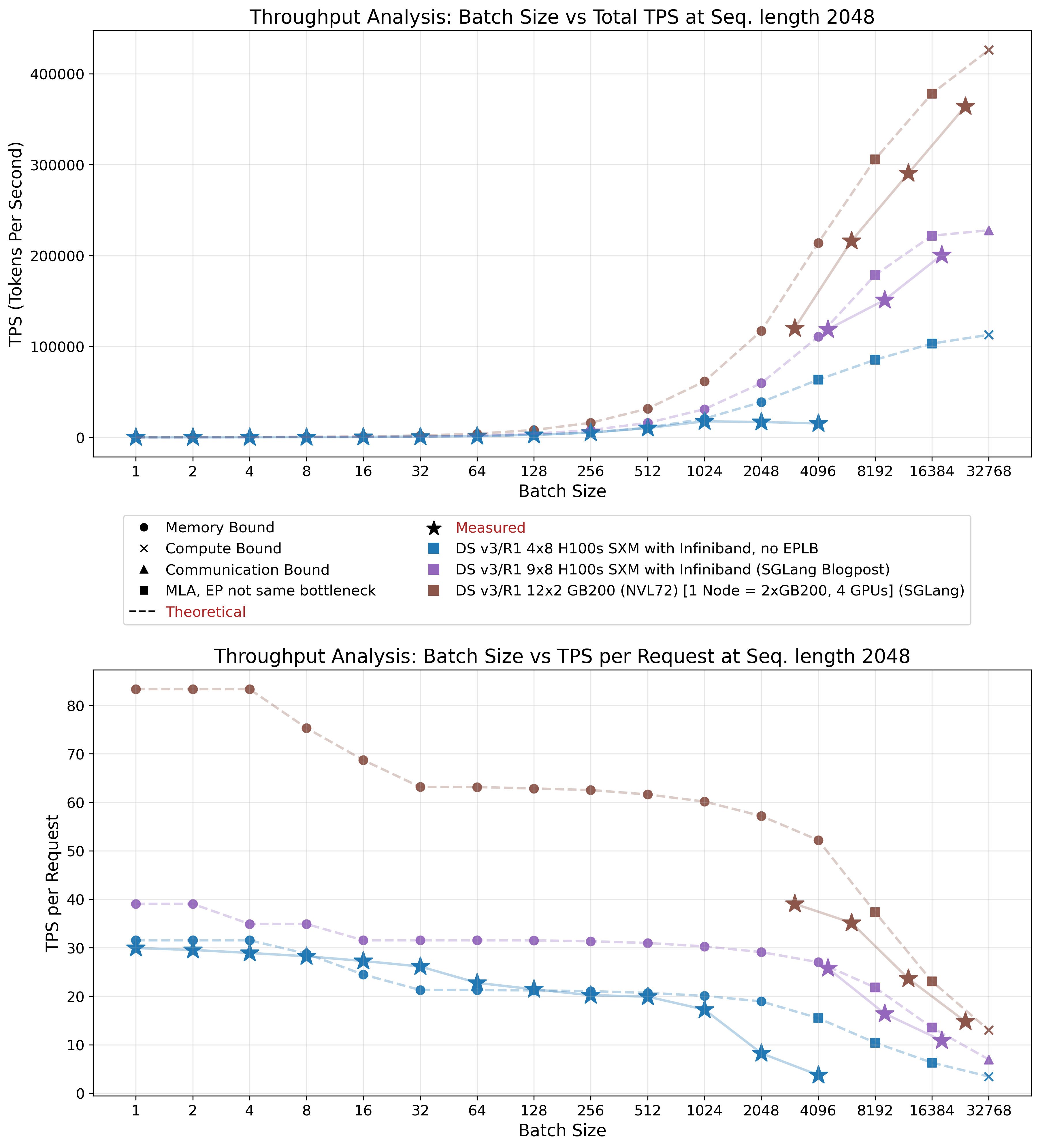
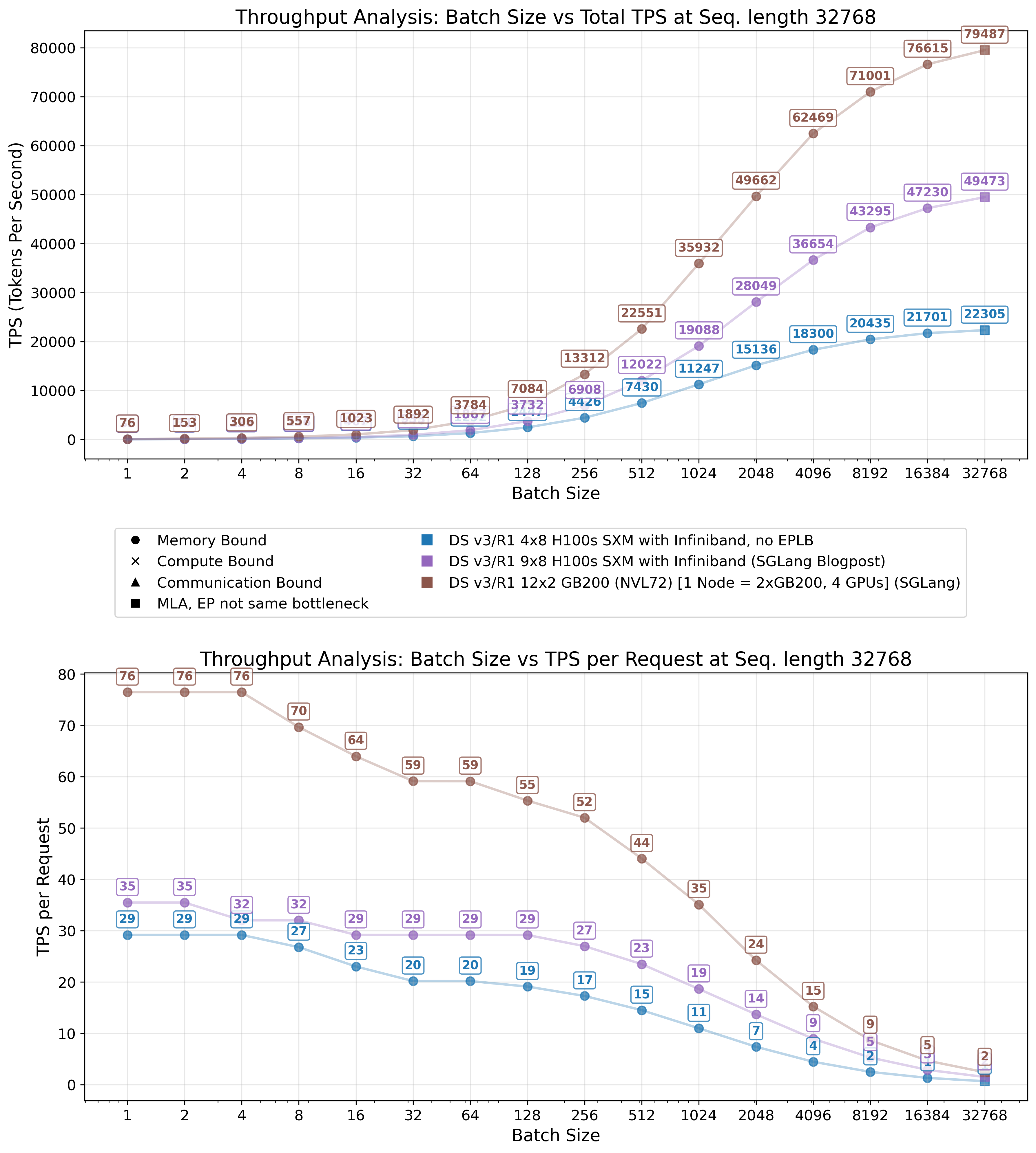
Figures 18 and 19 demonstrate that our theoretical model achieves reasonable agreement with empirical measurements. The first figure presents a systems total throughput and tokens per second (TPS) per request, while the second emphasizes efficiency by showing TPS per GPU.

As anticipated, our model overestimates actual performance by a considerable margin and we have to tune the model with our inefficiency factors. This discrepancy arises from two primary factors: first, individual component kernels fail to achieve peak performance as discussed previously; and second, peak performance of these individual components is rarely attained with constrained batch sizes. Furthermore, end-to-end optimization is often suboptimal, resulting in kernels optimized for different operational scenarios. These factors justify our incorporated inefficiency assumptions.

Small batch size estimation proved particularly challenging, as illustrated in Figure 18. At batch size 32, actual performance in our setup (shown in blue) exceeds theoretical predictions (given our inefficiency factors; it does not exceed the upper bound posed by the hardware itself). In our model, we assumed uniform expert activation probability, which does not reflect reality. In practice, fewer experts are activated, resulting in higher throughput than predicted. As batch size increases, throughput converges to predicted levels, indicating activation of most to all available experts.

Consistent with our stated assumptions, the model does not assess whether given batch sizes are practically feasible under given systems memory constraints. In our system configuration, sequence eviction begins after batch size 1024, causing a sharp decline in per-request throughput and total throughput saturation. Increasing node count expands the amount of memory available for KV cache, enabling larger batch sizes as demonstrated by the two SGLang configurations.

Figure 18: Comparing the theoretical model with real world measurements for decode throughput performance. The measurements for the 4x8 H100 setup were conducted using our tokenomics benchmark, running AIME requests against the model. Data for the two other setups stems from the SGLang two blogposts Our model works well in different scenarios on multiple hardware setups.

Throughput: Theory vs Practice

Examining Figure 19, we observe that increasing batch size per GPU improves system efficiency substantially. However, realizing these optimal batch sizes necessitates extensive memory allocation for storing KV cache. Given that total weight size remains largely static (excluding data-parallel MLA weights), distributing computation across additional GPUs reduces the per-GPU weight burden proportionally.

Figure 19: Per-GPU efficiency across all configurations demonstrates consistent scaling characteristics. Measurements on our system (in blue) exhibit a performance ceiling due to token memory constraints that trigger sequence evictions, preventing running the full batch concurrently. This limitation clearly illustrates that additional memory capacity would enable our system to achieve higher throughput levels, validating the case for larger setups.

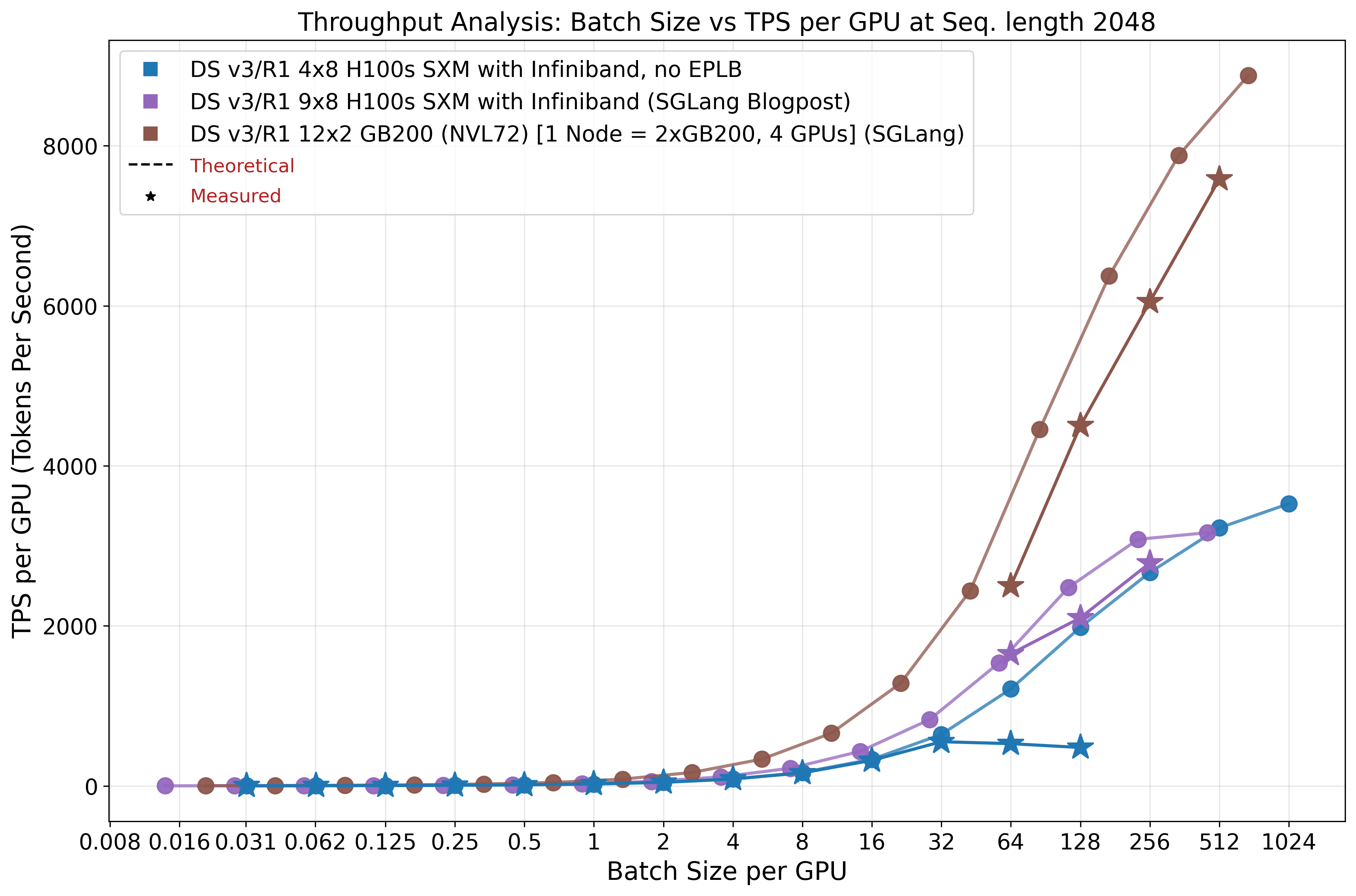
An increasing problem that large-scale systems pose is the communication overhead, which scales linearly with batch size. Consequently, configurations with large batch sizes and short sequence lengths may encounter communication bottlenecks. This phenomenon manifests in Figure 19 where the 4x8 H100 configuration achieves higher per-GPU throughput at batch size 512 compared to the 9x8 H100 setup, because the latter becomes communication-bound. Nevertheless, the former configuration cannot sustain these batch sizes in practice and will evict sequences, effectively running at smaller batch sizes. This also demonstrates the advantages of the NVL72 super node for inference workloads, effectively mitigating potential communication constraints.

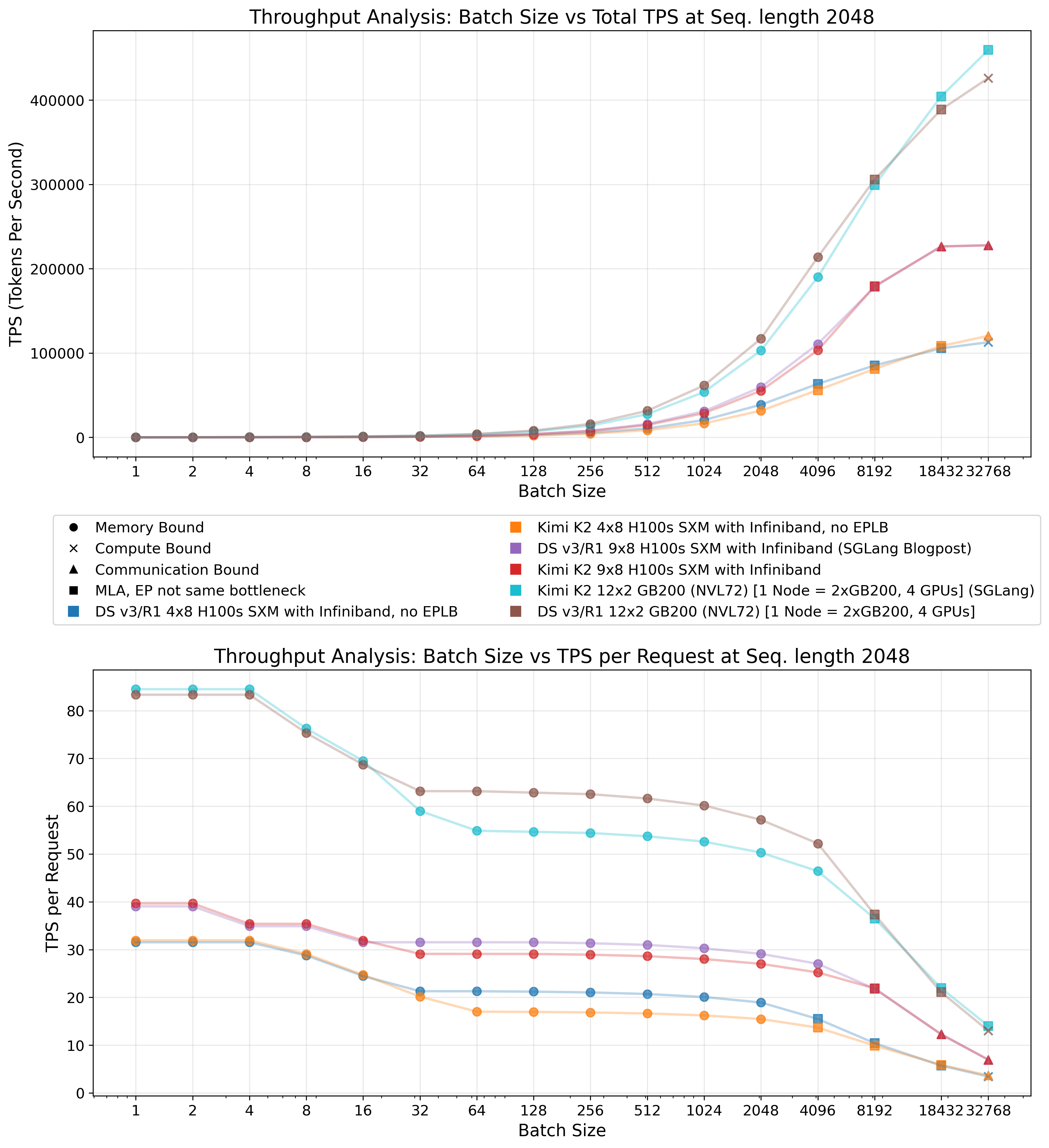
Kimi-K2 represents the first open-source LLM surpassing 1T parameters. The model employs the essentially identical architecture to DeepSeek V3.1, just with more routed experts per layer. As demonstrated in Figure 20, this configuration yields reduced throughput, particularly under memory-bound conditions where MLA runtime remains minimal. However, achieving equivalent batch sizes across identical hardware configurations is infeasible for large batches, as Kimi-K2 requires greater GPU memory allocation for storing its weights. Consequently, while theoretical performance degradation appears modest, practical performance disparities may be more pronounced due to reduced effective batch sizes compared to DeepSeek V3.1 deployment.

Figure 20: Comparison of theoretical predictions for Kimi K2 to DeepSeek v3. Even though Kimi K2 has a lot more weights, its only slightly larger due to the MLA and the communication being the same in both models. However, we dont model if a given setup would actually have enough memory and thus would be able to run a given batch size. Kimi K2 would reach this limit much earlier leading to more evictions and smaller achievable batch sizes.

Similar challenges with increased KV cache evictions and diminished effective batch sizes emerge when serving long sequences, as their KV cache demands substantial memory space. Although sequence length exerts a comparatively small impact on decode performance, as shown in Figure 21 (while exhibiting quadratic dependency during prefill on the sequence length), it constrains to running very low batch sizes, significantly reducing system efficiency.

For example, a 4×8 H100 setup provides roughly 20 GB of GPU memory per GPU for the KV cache. At a context length of 32,768 tokens, this translates to a maximum effective batch size of

\(\frac{20\times 10^9 \times 4 \times 8}{70\times10^3\times32768} \approx 279 \)

In practice, fragmentation of the KV cache and other inefficiencies reduce this number further. DeepSeek reports a much shorter average context length of 4989 tokens, which remains within manageable parameters.

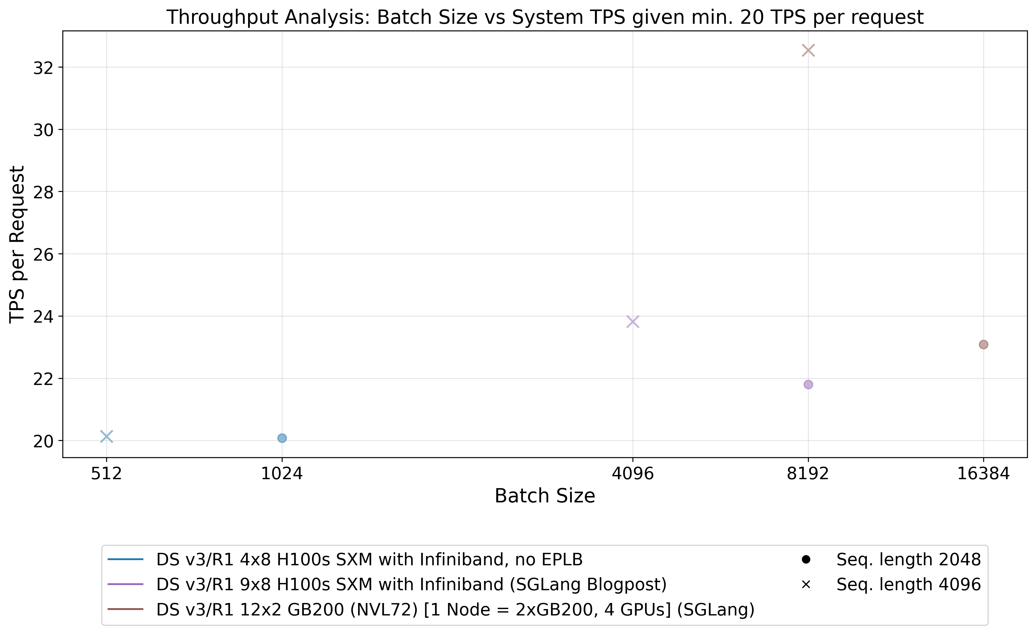
Production serving environments typically operate under service level agreement (SLA) requirements that mandate minimum TPS thresholds per request. As illustrated in Figure 22, these performance guarantees often impose surprisingly restrictive limits on achievable batch sizes. Providers find themselves constrained to operate with smaller batches to meet per-request latency requirements, resulting in suboptimal efficiency. This constraint disproportionately affects smaller deployment configurations, creating a natural advantage for large-scale enterprise operations, serving to hundreds of thousands of customers.

Our previous analysis has given limited attention to the prefill phase. During prefill, the system computes the complete KV cache for all input tokens and generates the first output token. The computational complexity of this phase scales quadratically with sequence length due to the full attention computation required. For shorter sequences, prefill duration remains substantially shorter than the subsequent decode phase. However, in long-context scenarios, prefill can exceed decode time, creating significant system bottlenecks.

Serving frameworks typically interrupt decode operations to process prefill batches, stalling the entire inference pipeline. Additionally, prefill operations are generally compute-bound rather than memory-bound, requiring distinct optimization strategies compared to decode. Large-scale deployments address this by implementing prefill-decode disaggregation, physically separating these phases across different instances. The prefill instance typically operates on fewer GPUs than the decode instance, reflecting the shorter duration and different resource requirements of prefill operations.

Figure 21: Serving long contexts affects decode performance less than prefill, since prefill’s runtime scales quadratically with input sequence length. However, a much bigger factor for decode, one we don’t currently model, is the size of the KV cache. A large KV cache renders the MLA memory bound for larger batch sizes and additionally forces running at smaller effective batch sizes, preventing the operation from becoming compute-bound in any realistic setup.

Figure 22: The plots shows the maximum achievable batch size for running with at least 20 TPS per request. This limit is arbitrary but seems close to what providers often offer as an SLA. Again the setup using the NVL72 outshines the competition, allowing for more efficient serving given an SLA.

Interactive chat applications and agentic workflows frequently involve multi-turn sequences where consecutive requests share common prompt prefixes. Given the potential length of these conversational contexts, repeatedly executing prefill for shared content becomes highly inefficient. Sophisticated caching mechanisms can drastically improve performance by reusing computed KV caches across requests. Effective caching architectures extend beyond GPU memory to use CPU memory and even persisting to disk. Even disk-to-GPU transfers often outperform recomputation for sufficiently long sequences. Additionally on-disk caches can be held for longer, potentially for days.

Such caching infrastructure can also serve as a buffer layer between disaggregated prefill and decode instances. Systems like LMCache and Mooncake provide foundational solutions to this problem. However, setting up such a caching infrastructure is non-trivial, and we save this topic for a future blog post. For the current analysis, we note that while prefill can substantially impact overall system performance, well-designed caching strategies offer substantial mitigation. DeepSeek's production deployment reports achieving approximately 56.3% cache hit rates, demonstrating a good reduction in prefill time when deployed.

While open source inference frameworks such as SGLang and vLLM may not achieve the absolute peak performance of specialized commercial inference providers like Fireworks or Together, we believe the performance gap remains relatively narrow. Evidence from production deployments, as referenced in Tweet 23, suggests that open source solutions approach state-of-the-art efficiency levels achieved by major enterprise implementations.

Figure 23: Member of technical staff at Thinky suggesting that the open-source inference software is not that far behind the proparitary inference software stacks available inside the big labs. Twitter

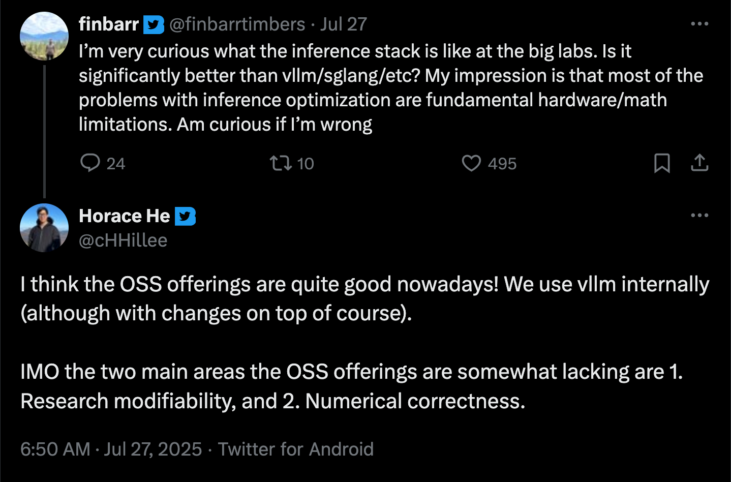
Our theoretical analysis combined with empirical measurements indicates that proprietary inference providers likely achieve comparable computational efficiency to well-optimized local personal deployments. However, these commercial providers maintain competitive advantages through access to superior hardware and more favorable economies of scale. The primary differentiation appears to stem from infrastructure advantages and economies of scale rather than fundamental algorithmic or implementation superiority in the inference stack itself.

Hardware considerations and profit margins

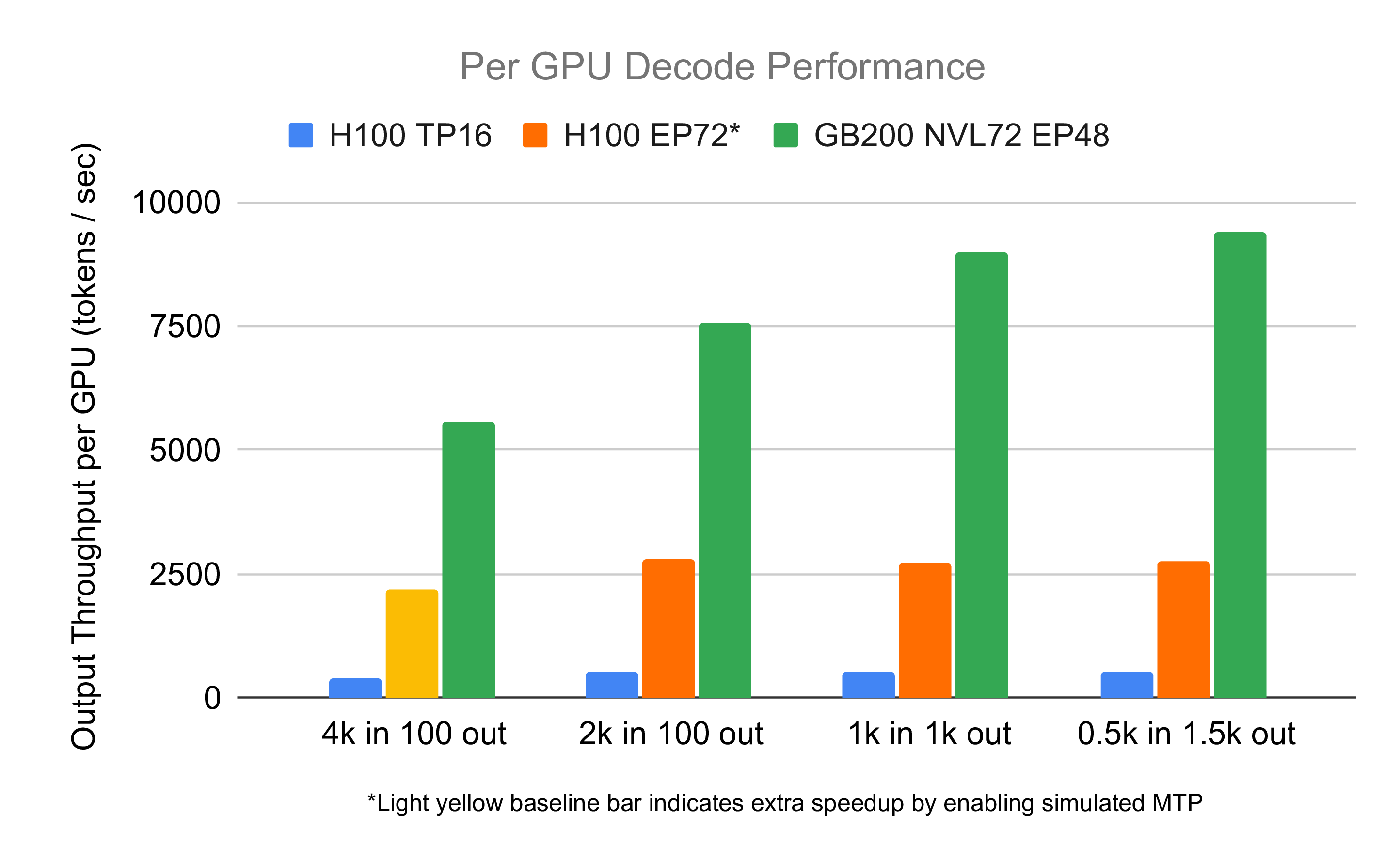
When deciding on hardware for large-scale MoE inference setups like DeepSeek V3.1 or Kimi, several key factors must be considered. First, due to the sparse computation pattern and its effects on the parameters that need to be loaded for a forward pass, there are significant economies of scale from adding more GPUs to the setup. In other words, a combination of four nodes should outcompete two pairs of workers running on two nodes. This is pretty well visualized in the graph created by the SGLang team (see Fig. 24), where a setup of 72 GPUs vastly outperforms one with 16 GPUs involved on a per GPU basis, an observation that confirms what we have seen before in results from Perplexity (see Fig. 2).

Figure 24: Token throughput measured on NVL72 SGLang Blog. 2.08.2025

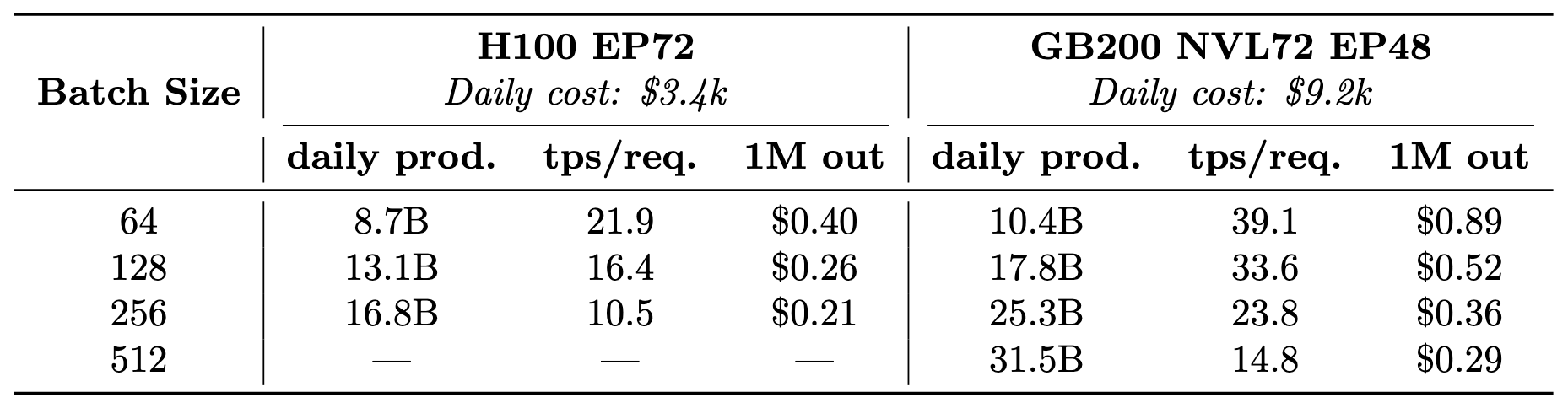
Second, cumulative throughput and per-user experience are highly dependent on the batch size at which the setup operates. This is well visualized in the benchmarks run we did for testing DeepSeek (see Fig. 18), and in the numbers provided by the SGLang team (see Fig. 25). The larger the allowed batch size the larger cumulative throughput but at a cost of worse "per user" experience (see Tab. 1) - a fundamental trade-off in inference optimization.

Figure 25: Token throughput measured on NVL72 SGLang Blog. The input and output lengths are set to 2000 and 100, respectively.

\(\begin{equation} \text{throughput per GPU} \times \text{number of GPUs} \times 3600s \times 24h = \text{daily token production} \end{equation}\)

\(\begin{equation} \text{H100 EP72 at bs 64} = 1400tps \times 72 \times 3600s \times 24h = \text{8.7B tokens/day} \end{equation}\)

\(\begin{equation} \frac{\text{throughput per GPU}}{\text{batch size}} = \text{throughput per request} \end{equation}\)

\(\begin{equation} \text{H100 EP72 at bs 64} = \frac{1400tps}{64} = \text{21.9 tokens/request} \end{equation}\)

\(\begin{equation} \frac{\text{daily operational cost}}{\text{daily token production (in millions)}} = \text{cost per 1M tokens} \end{equation}\)

\(\begin{equation} \text{H100 EP72 at bs 64} = \frac{\$3,456}{8,700M} = \$0.40 \text{ per 1M tokens} \end{equation}\)

Table 3: Daily production token production, tps enjoyed by each user, and cost per 1M output tokens. We only consider here the decode phase and leave prefill out of the scope for now. We assume the numbers from SGLang blogpost. The input and output lengths are set to 2000 and 100, respectively. At longer context these numbers will look differently, but we hope this table shows the scale of overcapacity. We assume $2/h and B200 at $8/h. Especially the second number is to be treated with cautious as there is no official market for NVL72, no provider offers this on demand so there is some guessing on our part here.

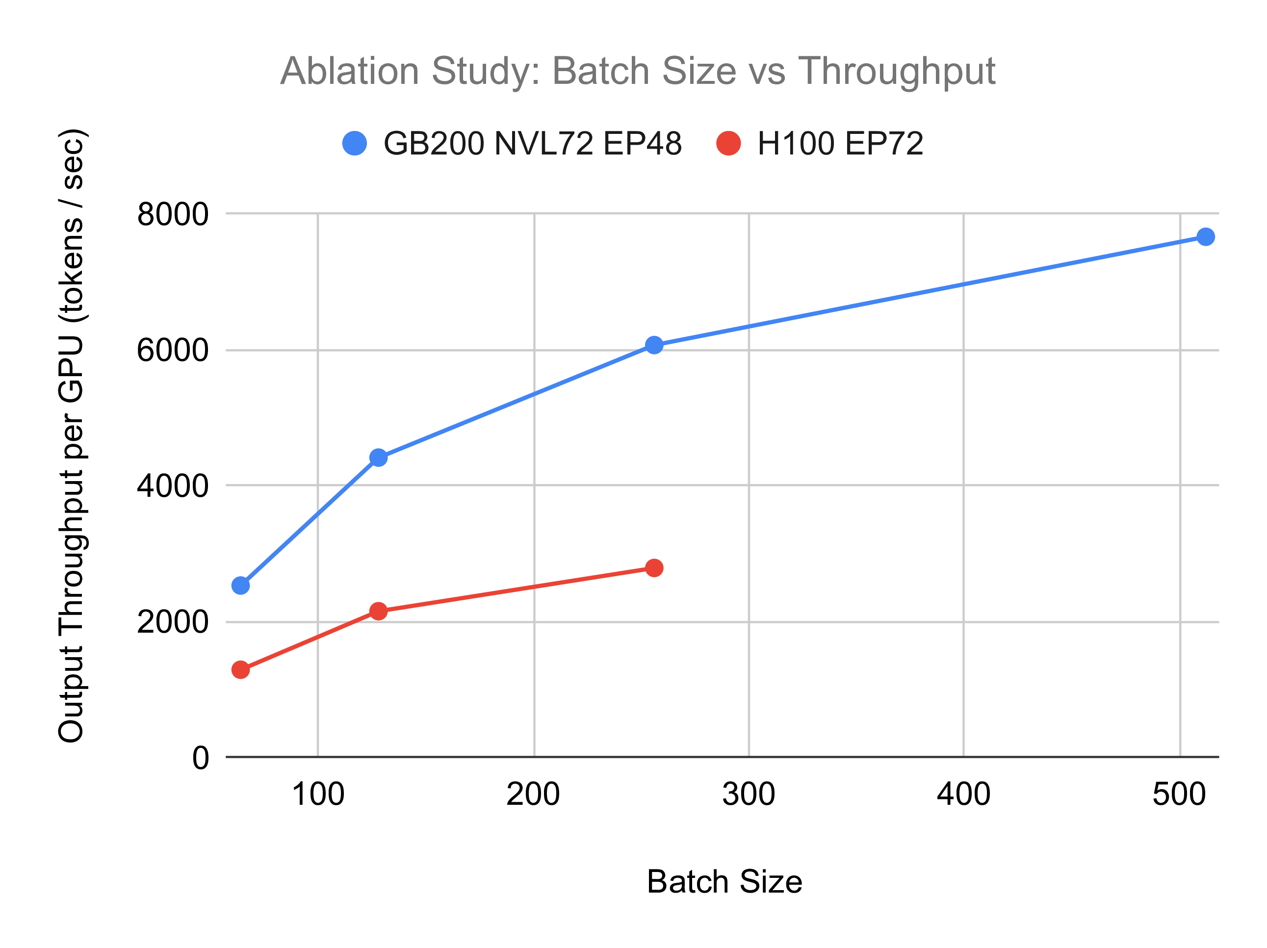
Hardware selection is the next critical consideration. The optimal choice is highly contingent on the latency/throughput requirements for your specific use case. While B200s in NVL72 will offer superior per-GPU performance compared to H100s, they come at a significantly higher price point - assuming you can even secure them³. Depending on what the inference provider wants to prioritize, either cost or latency, it will affect the type of hardware that will be optimal here.

For your exact application, how many input and output tokens do you run with, how big is your profit per user, how big is your spread in the number of concurrent users per day, how flexible are users, and at the time of peak usage, how low can the tps drop to? All of these factors should impact what hardware will be optimal for you.

One of the interesting observations we made after running the theoretical model for different hardware setups was how much of a bottleneck for B200 slow interconnect is. There seems to be a massive performance gap between the numbers we estimate for B200s connected via InfiniBand and the ones connected by NVLink. This is obviously highly contingent on the model and how much we communicate between the nodes, but overall we believe that for model of a scale such as DeepSeek, running on B200s might be actually suboptimal, as the coms overhead is taking away most of the gains we get from faster memory and more FLOPS compared to H100s (see Fig. 27).

Figure 27: Comparing a system based on the DGX B200 nodes to an NVL72 reveals a striking difference: The DGX systems gets communication bound due to relying on Infiniband for the inter-node communication, drastically limiting the performance compared to the NVL72 system.

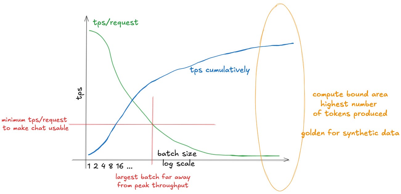
Another observation we hope you can take out from reading this text is how "chat centric" the current inference providers are. If you look at the throughput of DeepSeekV3 from various providers, as reported by OpenRouter, most of them offer very comfortable 50+ tps (see Fig. 28). While this is great if we have real time application like a chat, it is less than optimal if we want to use the model to generate the synthetic data. As we have seen multiple times throughout this text, in benchmark from Perplexity (see Fig. 5), in our theoretical estimations and in the real world observations we did (see Fig. 19), keeping the tps so high, while great for real-time applications, is suboptimal when we want to produce as large numbers of tokens as possible. For that the operational batch size would need to be largely increased. This would result in significantly degraded tps performance per request, but substantially higher overall throughput. For asynchronous or non-time-critical workloads, this trade-off is highly beneficial, dramatically reducing cost per token.

Figure 28: DeepSeek V3.1 speeds offered by various providers. 2.08.2025

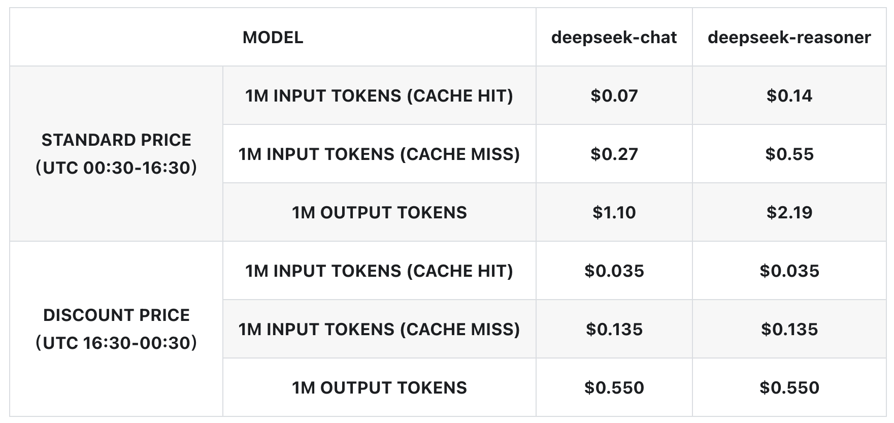
Such setup would be ideal for synthetic data generation, where individual latency is irrelevant and the goal is maximizing total token production per dollar of hardware investment (Fig. 29). However, we believe that the current inference providers inadequately serve this market. While some offer batch discounts - Fireworks provides 40% off batch APIs, DeepSeek offers 50% off-peak pricing in China (see Fig. 32) - these limited options suggest significant unmet demand for flexible, throughput-optimized serving.

Figure 29: Conceptual model showing the problem with using the same setup for synthetic data generation and real-time API.

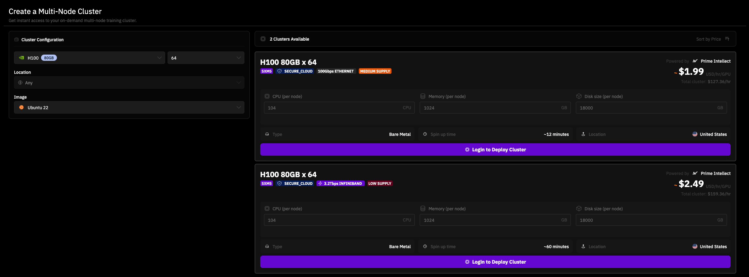
This infrastructure gap presents a significant opportunity for NeoCloud providers specializing in short-term, high-throughput compute rentals. Already today some providers, like Prime Intellect, offer on-demand access to the cluster of up to 64 H100s (see Fig. 30). Such a setup would be capable of daily generating billions of synthetic tokens even for large models like DeepSeek.

Reasoning traces from such data runs could be used for a reinforcement-learning fine-tuning (RLFT) in a product similar to the one offered by OpenAI. We believe that using RL to train models that directly maximize the business-specific rewards shows significant growth potential. Think of a virtual assistant helping people in making purchasing decisions, which is rewarded with actual dollar revenues, amplifying the actions that better convert into sales, or a virtual companion that promotes deeply engaging conversations, keeping users longer in the app. There undoubtedly is a huge economic incentive for businesses to apply such techniques, maximizing the revenues in a similar way as YouTube or TikTok already do with recommendation engines.

Figure 30: H100 multi-node cluster available at Prime Intellect. Cluster of InfiniBand connected nodes costs $2.49 × 64 ≈ $160/h or $160/h × 24 = $3825/day. We estimate such cluster to be able to produce up to 30B synthetic tokens within a day.

Furthermore, to improve the inference economics, such RL models could be trained using LoRA adapters or a similar technique and served alongside thousands of other models, all catered to specific use cases. This multi-tenant serving approach represents a compelling business opportunity for inference providers. Clients hosting their custom LoRA adapters on a provider's infrastructure face significant switching costs when migrating to competitors, as the adapters are optimized for specific serving configurations and client workflows. RLFT is based on unique and nuanced rewards that are very client-specific; unlike standard supervised fine-tuning (SFT), it much much more challenging to replicate it just via in-context learning, making it an even more compelling case for inference providers.

We expect the inference markets to further specialize in regard to offered throughput, latency, and pricing. It is only natural for providers of super-fast tokens like Groq and Cerebras to command a much higher premium for the tokens they deliver at few-second latencies and for other providers like NeoCloud specializing in high-latency, high-throughput inference scenarios focused on synthetic data generation. We hope to elaborate on this space in the future text.

From Tokens to Dollars - Estimating Tokenomics

Now we can finally address the original question: What is a fair price per DeepSeek V3.1 token? As we hope you know after reading through this text, the answer is an unsatisfying it depends.

The price per token depends on two factors: how much our hardware costs, and how many tokens it can produce per unit of time. As shown in numbers from Perplexity (Fig. 5) and SGLang results (Fig. 24), there are significant benefits to the performance per GPU when more GPUs are deployed. Putting more GPUs into serving a large-scale MoE model will yield higher performance per GPU and, as a result, lower our costs and boost profits.

Moreover, since LLM inference is heavily memory-bound, the batch size at which we serve the model significantly affects the combined throughput across all requests. The larger the batch size we use, the more tokens we cumulatively produce, but this comes at the cost of increased latency for each individual user, as reflected by Tab. 3.

Furthermore, not all hardware is created equal. While B200s will offer superior compute GPU performance compared to H100s, they are significantly more expensive (see Tab. 3), making them likely a less optimal option when optimizing for cost efficiency and producing as many tokens as possible while minimizing costs

All in all, while we cannot provide an exact number, we hope this analysis provides valuable insights into the factors impacting token pricing. The theoretical performance model we provide, though not perfect, should offer solid intuitions about expected performance and the trade-offs between different hardware options.

The missing tokens

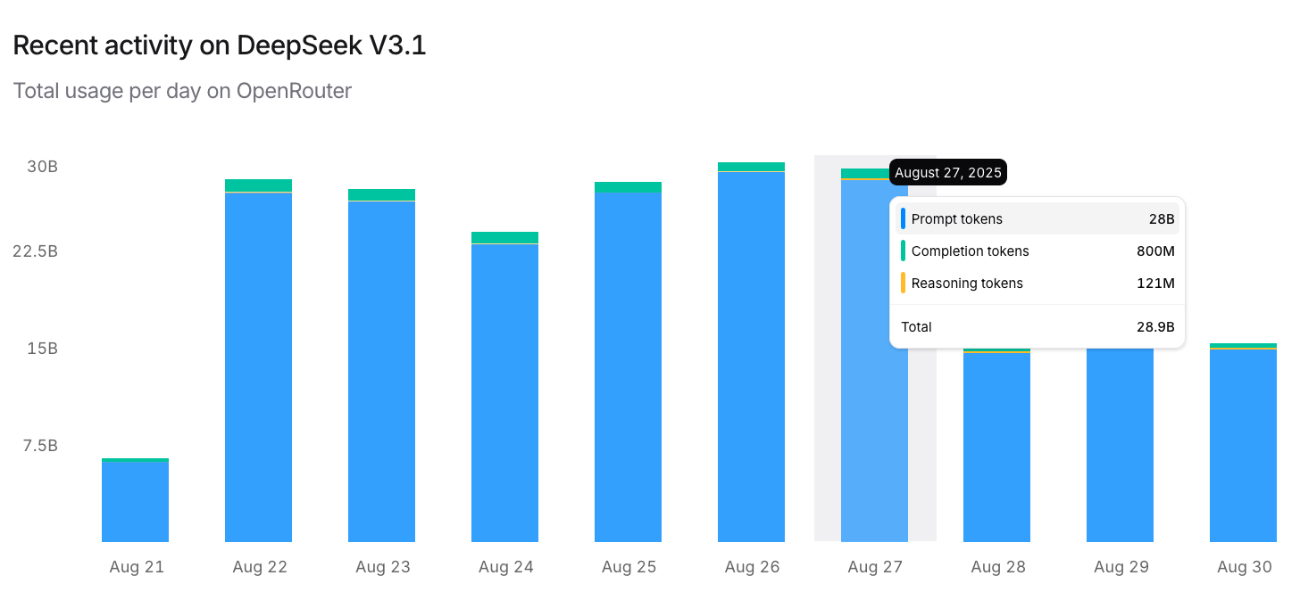
Finally, we want to address the elephant in the room: the problem of missing tokens in the global market. As of this writing, DeepSeek V3.1. remains the most popular open-source model on OpenRouter. While displayed daily consumption hovers around 30B tokens per day, upon closer inspection it becomes clear that the majority of these are input tokens, not output tokens. Daily global consumption of DeepSeek V3.1 output tokens on OpenRouter is approximately 1B tokens. A quick examination of our numbers in Table 3 reveals that with a fraction of a single NVL72, we could meet this demand 20 times over while maintaining a reasonable >30 tokens per second per request.

Figure 31: Daily DeepSeekV3.1 token production on OpenRouter. 30.08.2025

This is a pretty significant gap. How is it possible that the global consumption of the most popular open-source model is so small that it could be met by a single NVL72 with 20 times the capacity to spare? Given this low demand, how can so many inference providers sustain their businesses? Put simply: who is making money here?

One might argue that we only account for the decoded tokens and that the majority of income comes from the input tokens. We do this because, due to the caching mechanism, it is quite challenging to accurately estimate how big portion of input tokens cost can be captured by the inference providers.

To quote DeepSeek:

Within the 24-hour statistical period ... Total input tokens: 608B, of which 342B tokens 56.3% hit the on-disk KV cache.

Caching drastically reduces the cost of prefill, slashing times to first token, and enabling the inference provider to move nodes from doing prefill to only working on decode. For example, DeepSeek offers a 75% discount (see Fig. 32).

Assuming that the DeepSeek caching numbers hold across the industry, this would put the daily total profit achieved via OpenRouter at:

\(\begin{equation} \text{Input tokens} + \text{Output tokens} = \text{Cached input} + \text{Cache miss input} + \text{Output tokens} \end{equation}\)

\(\begin{equation} \text{Daily Profit} = (28 \times 1000 \times 0.56 \times \$0.07) + (28 \times 1000 \times 0.44 \times \$0.27) + (0.800 \times 1000 \times \$1.1) \end{equation}\)

\(\text{Daily Profit} = \$1,097.60 + \$3,326.40 + \$880.00 = \$5,304.00\)

spread across all of the inference providers. Some providers don't offer caching, some offer cheaper pricing, and some offer more expensive pricing than DeepSeek so estimating the exact amount being spent daily is difficult, but we don't expect it to be much different than that. Which begs a question? Where is the demand for DeepSeek?

The first natural answer is that OpenRouter just captures only a small portion of the global demand for DeepSeek models. The question is, how small?
Even had it been just 1%, assuming that our estimations are accurate, it could easily be fulfilled by 3 to 4 NVL72s. One caveat of this calculation is that our numbers (based on the SGLang benchmark) assume a short input length of 2000 tokens, something that we try to account for in our theoretical model. If we increase the context length from 2k to 32k the KV cache footprint increases 16x, severely limiting the batch size at which we can operate, considerably altering our potential margin.

Overall we don't have an answer backed by precise data for the question "where are the missing tokens?"; In the numbers revealed by DeepSeek, they claim to be processing 168B output tokens a day (these numbers are from Feburary 2025, the current numbers are likely significantly higher). This is orders of magnitude more than OpenRouter, a gap that we find quite surprising, but that would largely answer this question. Perhaps the vast majority (>99.9%) of the global demand for the DeepSeek tokens is matched by calling the providers directly and not via services gathering multiple providers.

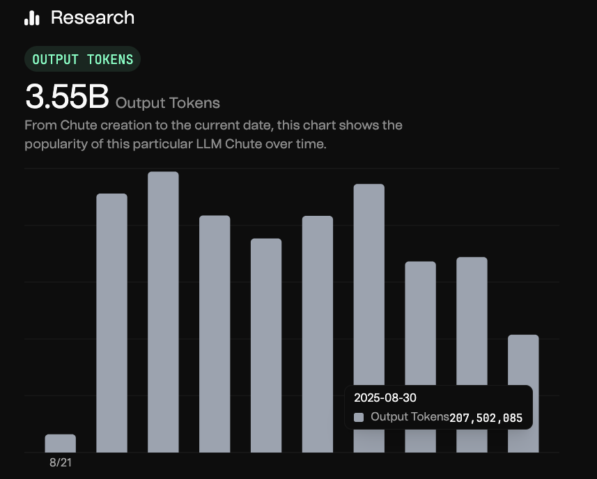
The only other provider that we were able to find to openly share their numbers is Chutes (see Fig. 33). At around 0.2B output tokens and much lower pricing (only 80¢/1M output tokens), they generate an estimated daily income of $160 from output tokens of DeepSeek V3.1⁴. On top of that, they seem to generate significantly more income from input tokens, but this seems to be mostly due to lack of caching. With the emergence of easily accessible caching solutions, such as LMCache and Mooncake, it is something we expect to be solved in the coming months, with the resulting savings being passed onto consumers.

Figure 32: DeepSeek API pricing, Caching offers substantial savings of (1.0-7/27)=~75%. Note that deepseek-chat and deepseek-reasoner are the same model - DeepSeek V3.1, just with the reasoning setting on or off. 30.08.2025

Figure 33: Daily DeepSeekV3.1 token production on chutes. 30.08.2025.

While talking to industry insiders, it was suggested to us that some leading inference providers, those that have raised nine-figure funding rounds, are processing trillions of tokens daily, but as of September 2025, there is no publicly available evidence supporting such claims. We find this dichotomy between Google, ByteDance, or MSFT declaring that they are processing trillions of tokens daily and the minuscule numbers we see for open-source providers to be quite perplexing!

Acknowledgements

Thanks to @felix_red_panda for giving it a read before the publication, and bouncing out the ideas

1. We elaborate on this in a later part of the text

2. See our previous article on for the detial of TP.

3. While investigating this topic with industry insiders, we learned that due to extremely limited supply, securing NVL72 is close to impossible at the moment.

4. Please note that for some reason, DeepSeek R1 and V3 0324 remain much more popular on chutes, with a combined output token production of ~2B tokens a day as of of 30.08.2025.