Why are embeddings so cheap?
or a lesson in profiling and FLOPS per dollar

Embeddings are a fundamental component of every modern retrieval augmented generation (RAG) system. State-of-the-art (SOTA) embeddings are provided by companies such as OpenAI or Google at prices up to two orders of magnitude lower on a per-token basis than prices for generative models such as GPT or Gemini. In this analysis, we show what computations are required to produce an embedding and how, based on these computations, we can derive the true dollar cost of processing a token.
Our contention is that since the cost of processing a token is so minuscule and all embedding models converge to similar semantic representations, this means that no provider enjoys a sustainable moat. This results in underlying low costs being passed directly onto the consumers, driving prices to rock bottom.
As we demonstrate, with sufficient demand and scale, the price to process a million input tokens can be driven below 1¢ for SOTA embedding models topping the evaluation leaderboards.
The insight we hope you take from reading this analysis is that, unlike GPT-style autoregressive models, modern embedding models are primarily compute-bound, not memory-bound, meaning they largely don't benefit from batching. We show that FLOPS/dollar is the key hardware parameter for optimizing cost structure when building an embedding API.
The remaining sections proceed as follows. First, we estimate the FLOPs of a forward pass based on model architecture, comparing these FLOPs with the cost of loading the model from global memory. Then we benchmark a real-world embedding inference system, showing how quickly computations saturate our system and how little additional utilization we gain from batching. Finally, we dive deep into CUDA profiling, examining which kernels are invoked and profiling them in detail to identify system limitations.
We assume that the reader is familiar with the concepts presented in our previous text: LLM Inference Economics from First Principles. Before proceeding to read this, the reader should be familiar at a high level with how transformer models work, what it means to be compute- or memory-bound, what the FLOP is, and how many FLOPs there are in a matrix multiplication. We highly recommend you get familiar with these concepts first, as we will be building on top of this understanding. If you are unfamiliar with these concepts, please read the previous text first.
Introduction
Embedding models transform sequences of data, typically text or images, into semantic representations. These representations take the form of high-dimensional vectors that capture meaning across different dimensions.
This semantic representation can be later used in downstream tasks, such as “find me the document semantically similar to the question my user is asking”. Similarity is computed using linear algebra operations such as dot products or cosine similarity between vectors. While there exist some limits to what can be captured in this kind of single vector representation embeddings remain the fundamental block of any modern RAG system.
One of the first companies to offer the semantic embedding as an endpoint was OpenAI, back in December 2021. Since then, their embedding models have been updated and competitors like Google and Cohere have launched their own offerings, though OpenAI remains the market leader.
What is pretty special about the embedding endpoints is how cost-efficient they are to use. While OpenAI is charging up to $15/1M input and $60/1M output tokens for their O1 reasoning model1, embedding models are offered at an astonishingly small 10 cents/1M input tokens for the most popular `text-embedding-ada-002` model (see Fig. 1).
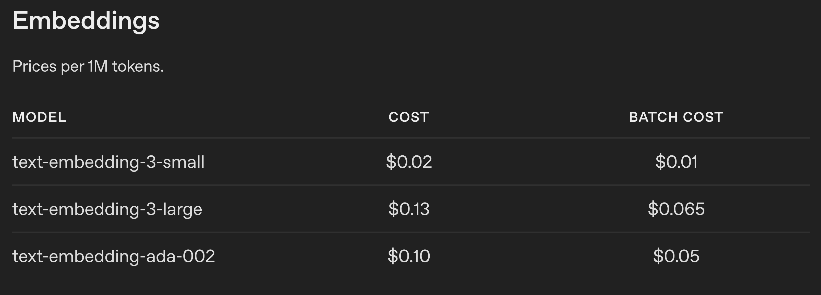
To illustrate how cheap it is, embedding the entire English Wikipedia corpus would cost approximately:
5B words or ~10M pages of text for $650.
If we look at the offerings from other competitors, the prices are mostly within a ballpark of this, with Google's gemini-embedding-001 at $0.15/1M input tokens and Cohere’s Embed 4 at $0.12/1M input tokens.
While these prices might appear as artificially low if we "count the FLOPS," we can clearly see that they are reflected in the underlying cost structure of processing a token. Generating an embedding is just extremely cheap, and these savings are passed directly onto the consumers. There's another factor driving prices down: embedding models are converging to similar semantic representations regardless of their architecture. If all models capture semantics similarly, differentiation becomes nearly impossible. This makes serving raw embedding a terrible business to be in and forces companies that used to specialize in this to pivot more towards the end-to-end search services that can command higher margins.
Qwen3 Embedding architecture
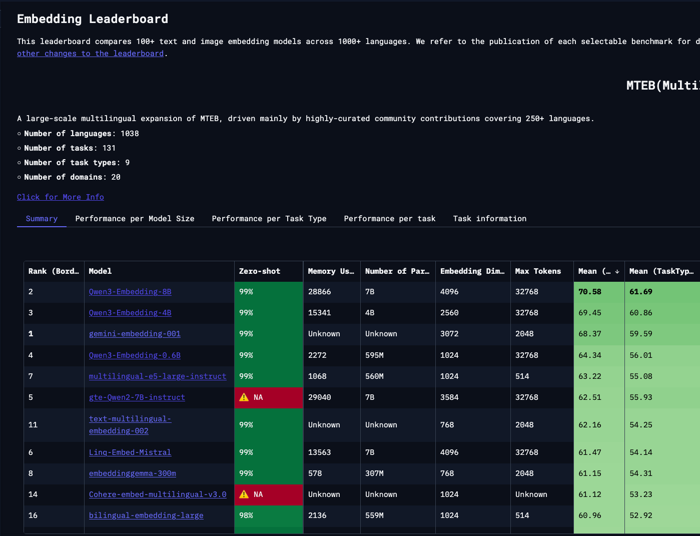
For our analysis, we use Qwen3-Embedding-8B as our example model. As of September 2025 it is a model topping the embedding tasks leaderboards (see Fig. 2). While many people validly point out the limitations of the real-world usefulness of using MTEB as a proxy for model quality, due to models overfitting on test data, it remains widely adopted. Since we don’t care that much about the exact model performance but more about the compute cost of generating an embedding representation, it should not be a problem for our analysis.
We make several key assumptions about commercial embedding models. We assume that closed-source models like text-embedding-ada-002 and gemini-embedding-001 share similar architectural designs with Qwen3. Specifically, we assume they are dense transformer models that produce embeddings via a single forward pass and are relatively compact at under 10B parameters.
The architecture of Qwen3 embedding is very simple, to quote the Qwen team:
The Qwen3 embedding … models are built on the dense version of Qwen3 foundation models and are available in three sizes: 0.6B, 4B, and 8B parameters. We initialize these models using the Qwen3 foundation models to leverage their capabilities in text modeling and instruction following.
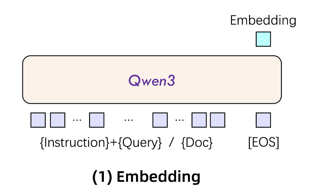
For text embeddings, we utilize LLMs with causal attention, appending an [EOS] token at the end of the input sequence. The final embedding is derived from the hidden state of the last layer corresponding to this [EOS] token.
This means that generating an embedding requires only a single forward pass through the model, extracting the hidden state corresponding to the final [EOS] token (see Fig. 3). In other words, embedding has (nearly) exactly the same compute footprint as completing the prefill phase, or producing the first output token, when using the auto-regressive version of Qwen3.
Counting FLOPs
*Please be aware that FLOPS and FLOPs mean different things. FLOPs (small s) is the plural of floating-point operations not considering time at all, but FLOPS (capital S) means floating-point operations that happen within a second.
In the previous text we estimated the total FLOPs of a forward pass of a Llama model at:
Where S is the sequence length of the processed sequence.
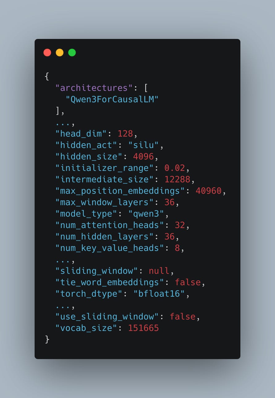
Qwen3 and Llama3 share a very similar architecture. Both are dense causal transformer models; both use group query attention and the silu activation function for MLP. One minor difference is that the ratio of hidden_size to intermediate_size is 3 (12288/4096, see Fig. 4) compared to Llama’s 3.5, though it is such an insignificant difference that we proceed to use the equation above to estimate the FLOPs of a forward pass of Qwen. For further details, please refer to the previous article.
Since for embedding representation we just use the hidden state of the last layer corresponding to the [EOS] token, this means we don’t need to calculate the probability distribution over the next predicted token, aka the LM head, meaning we can remove the FLOPs for calculating it. There are some extra FLOPs involved from the pooling layer, but for the sake of simplicity we skip them, as they involve very few operations. Bringing the total in a forward pass to:
Assuming we are processing S=1024 tokens and using the Qwen config as in Fig. 4 (num_hidden_layers=36, hidden_size=4096, num_attention_heads=32), we can quite easily estimate the total FLOPs at:
Using this, we can easily estimate the upper bound of how long it takes to process a sentence of 1024 tokens. To do so, we need to look into the FLOPS and memory bandwidth of a GPU. Performance can be capped either by us having to do too many operations (compute-bound) or by a need to load too much data (memory-bound).
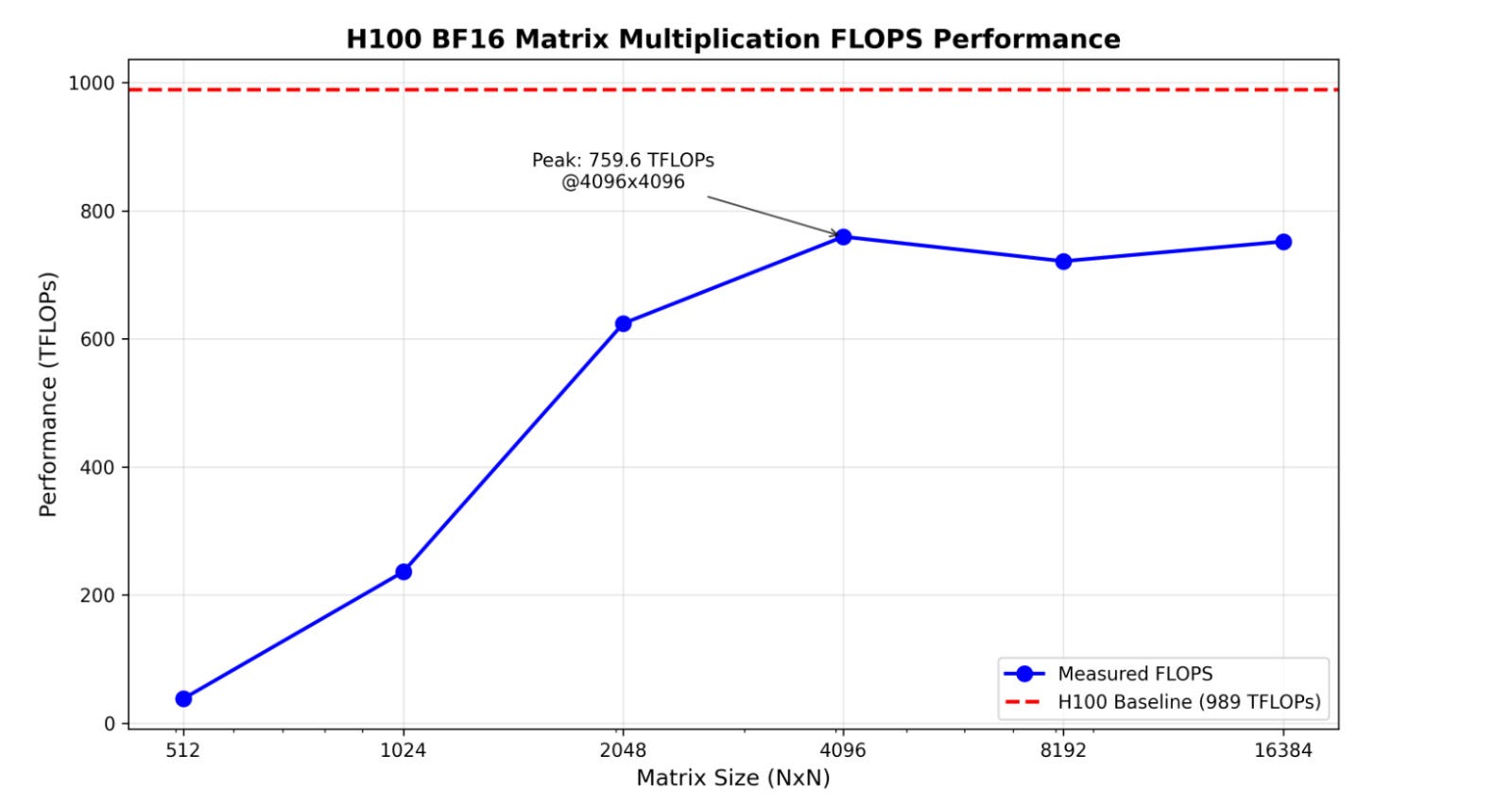
On paper NVIDIA H100 SXM5 delivers 989 TFLOPS of compute for BF16 with accumulation in FP32. It also features a fast high bandwidth memory (HBM) offering up to 3.3 TB/s throughput. However, in practice, due to the power constraints, H100 is not capable of actually achieving these declared FLOPS. As Horace He explains:
This observation that GPUs are unable to sustain their peak clock speed due to power throttling is one of the primary factors that separates “real” matmul performance from Nvidia’s marketed specs.
The figure that Nvidia provides for marketing is:
\(\text{FLOPS} = \text{Tensor Cores on GPU} \cdot \text{Max Clock Speed} \cdot \text{FLOP per Tensor Core Instruction}\)For example, on an H100, there are 528 tensor cores per GPU (4 per SM), the max clock speed for these is 1.830 Ghz, and the FLOP per tensor-core instruction is 1024. Thus, we have
1.830e9 * 528 * 1024 = 989 TFLOPS, exactly Nvidia’s listed number.However, you can only achieve this number by sustaining 1.83 Ghz clocks, and as we’ve seen above, the GPU just doesn’t have enough power to do that!
In our tests we achieved ~750 TFLOPS in matrix multiplication (see Fig. 5) on H100 SXM, varying with matrix dimensions. As we will show later, most of the time in calculating embeddings is spent in large-scale matrix multiplications - hence this will be a pretty good indicator of the realistic end-to-end performance we can expect.
To calculate an embedding, we need to:
Load the model weights once from global memory
Complete a forward pass involving ~16.4 TFLOPs of matrix multiplications and other calculations.
The model size can be easily estimated based on the number of parameters at:
meaning that a single model load takes around:
Meanwhile, when we do all 16.4 TFLOPs worth of calculations we estimated above, we will wait approximately
In practice the memory loading and computations on a GPU are to some degree overlapped, meaning that the factor limiting our performance will be the larger of these two times - compute in this case, or in other words, our calculation will be more compute than memory bound.
Assuming 0.021s for a single forward pass, we can estimate the upper bound of embedding throughput as:
In practice, we won't achieve these exact numbers. Both memory and compute figures represent theoretical upper bounds. Real-world performance falls short due to factors like imperfect memory-compute overlap, kernel launch overhead, and various computational inefficiencies.
Real world benchmark
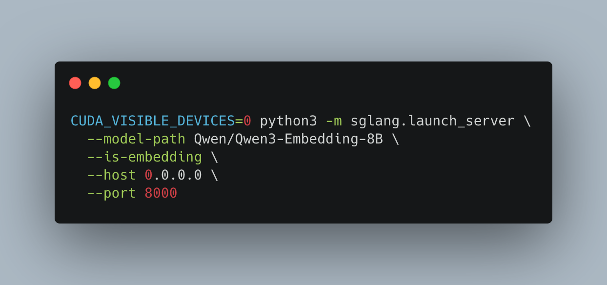
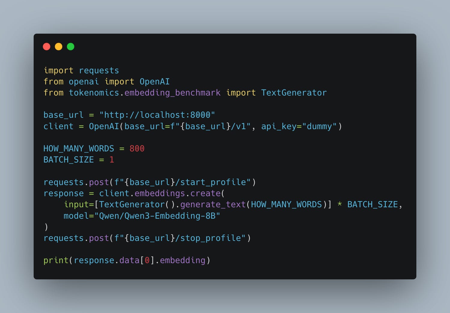
To measure the real-world performance of an embedding model, we can use the popular LLM inference engine - SGLang. Running it is quite simple (see Fig. 6) and should work out of the box on any H100 setup. SGLang provides an efficient inference platform, realized in the form of an OpenAI-compatible endpoint, and should be a good basis for our experiments.
We implemented a simple benchmark measuring inference engine response times. The benchmark takes two inputs: sequence length (in tokens) and batch size (simulating concurrent users). We sent batches of requests with predefined lengths to the API and measured processing time.2
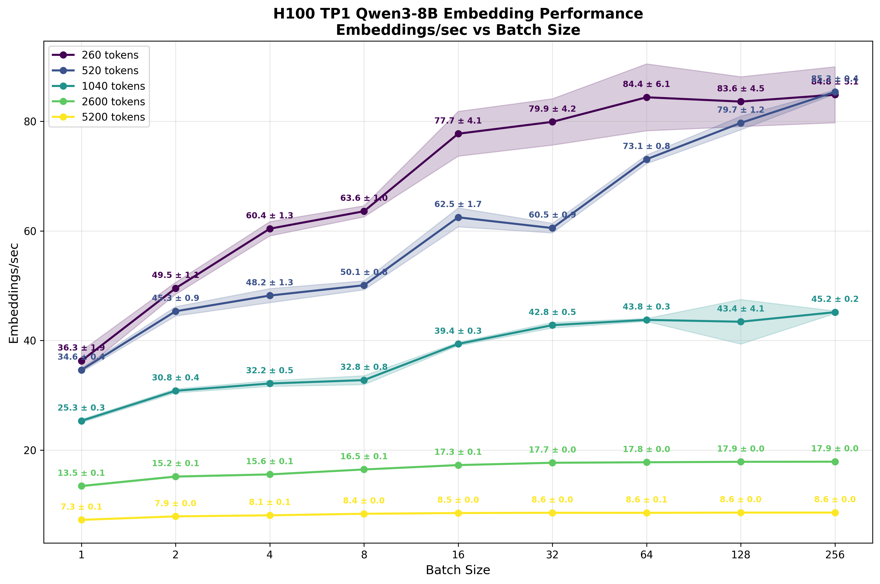
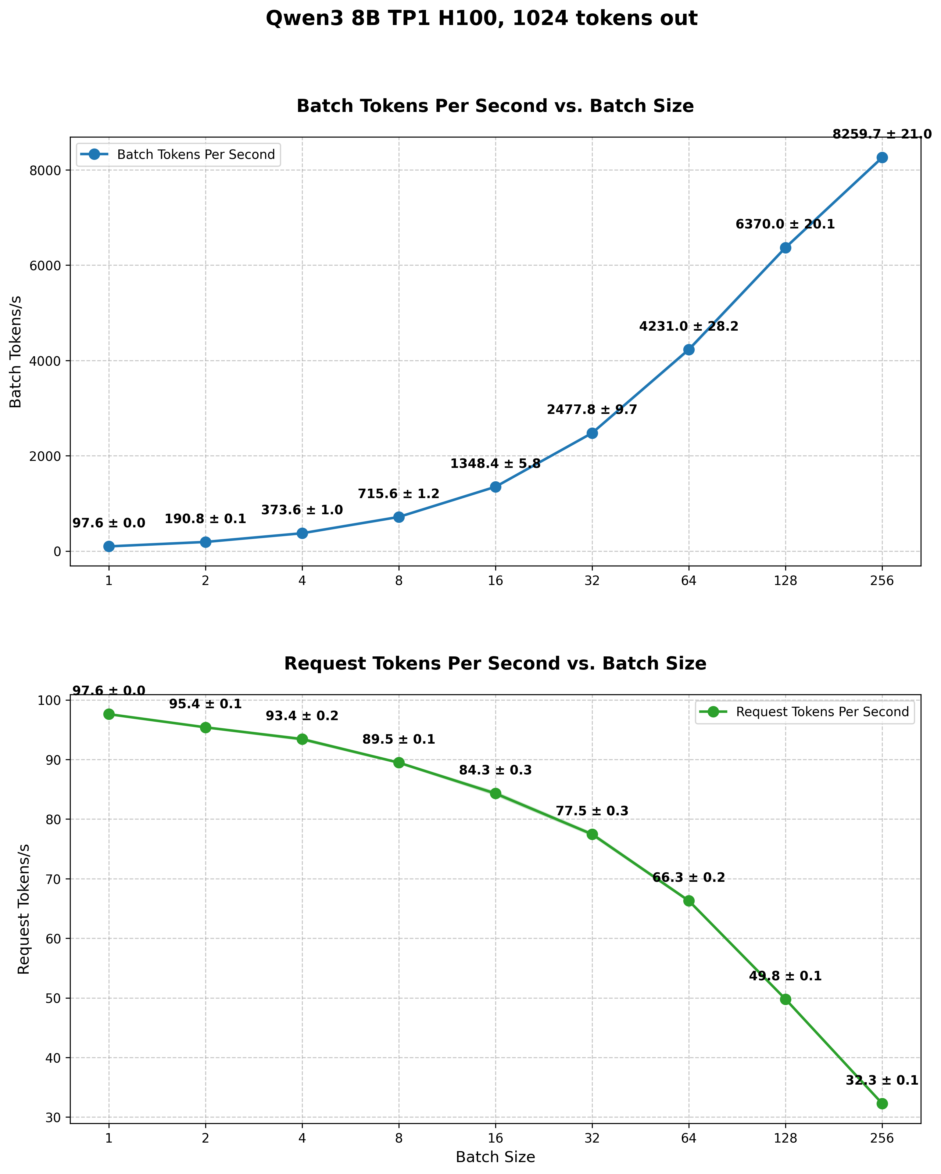
What the reader should immediately spot is how, despite batch size increasing, the number of embeddings processed within a second doesn’t scale significantly. For shorter sequences (260 and 520 tokens), increasing batch size from 1 to 64 yields only ~2.3x improvement in total token throughput. As sequence length increases and compute becomes more saturated, this scaling benefit diminishes ever further. For the longest sequences (5200 tokens), larger batch sizes provide virtually no benefit.
The reason for this situation can be largely explained by the FLOPS calculations we did above. We estimated that for batch size=1 and sequence length S=1024 tokens, the upper bound is ~47 embeddings per second, roughly double (47/25.3=1.86) what we observe in practice3. This gap is to be expected, as model calculations have extra overhead from launching multiple kernel grids, the lower arithmetic intensity of some kernels, and other inefficiencies.
Even at batch size=1, the computational workload substantially saturates the compute units. At larger sequence lengths, we're operating on increasingly large matrices with no spare compute resources available—the streaming multiprocessors (SMs) are fully occupied. As batches grow larger or sequences get longer, kernel launch overhead becomes a smaller fraction of total time, with most cycles spent on the calculations themselves.
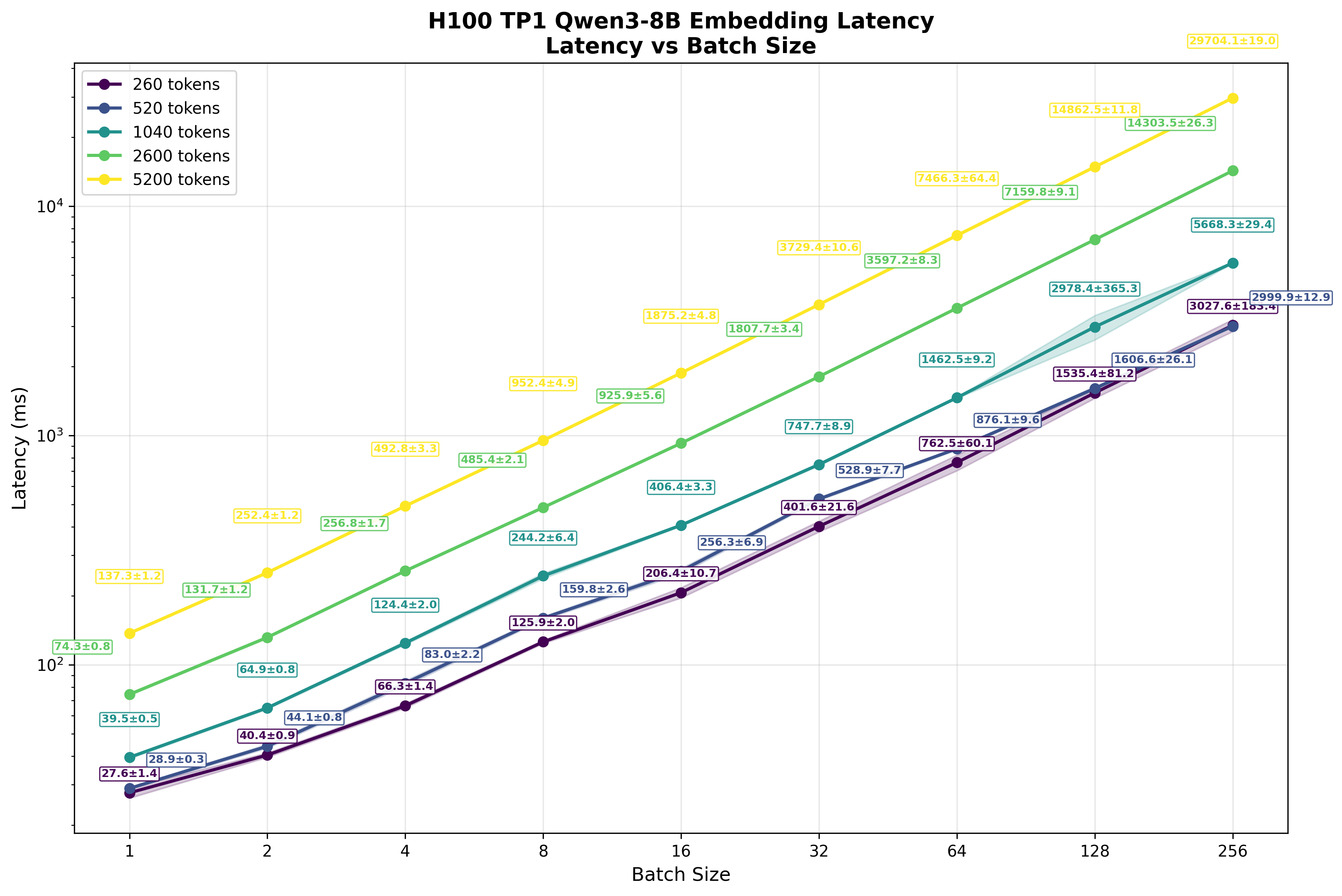
What you need to remember, though, is that since we are compute bound and we only get marginal improvements in the number of embeddings processed with increased batch size, it has a severe impact on the latency experienced by each user. Since we do these larger and larger scale matrix multiplications, they take longer and longer to finish. This represents a traditional tradeoff in LLM inference - combined throughput vs. the latency experienced by each user.
This contrasts sharply with autoregressive token generation. Here, because our computation is primarily memory rather than compute bound, increasing the batch yields substantial throughput gains. As Figure 9 shows, batch size increases correspond to significant improvements in overall throughput across all requests. The latency penalty for individual users is far less severe than with embeddings.
Text generation's memory-bound nature creates this favorable scaling. We primarily wait for model weights to load for each token generated while compute resources remain underutilized. Loading the model once and "sharing" this cost across multiple users has minimal impact on per-user experience.4
The fundamental difference lies in computational bottlenecks. While autoregressive generation is limited by memory bandwidth and benefits from amortizing memory costs across batches, embeddings face the opposite constraint. Embedding generation requires only a single forward pass, but this pass involves large-scale matrix operations that fully saturate available compute. This is the main intuition we hope the reader takes out of this text. Embeddings are primarily compute bound. Due to this there is only limited benefit to batching, and it comes at the cost of severely increased latency experienced by each individual user. This means that, unlike in serving GPT-style models, there are very limited benefits to scale - running big batches doesn’t slash our cost “per user”. This further decreases the appeal of serving embeddings as a business.
What profiling reveals
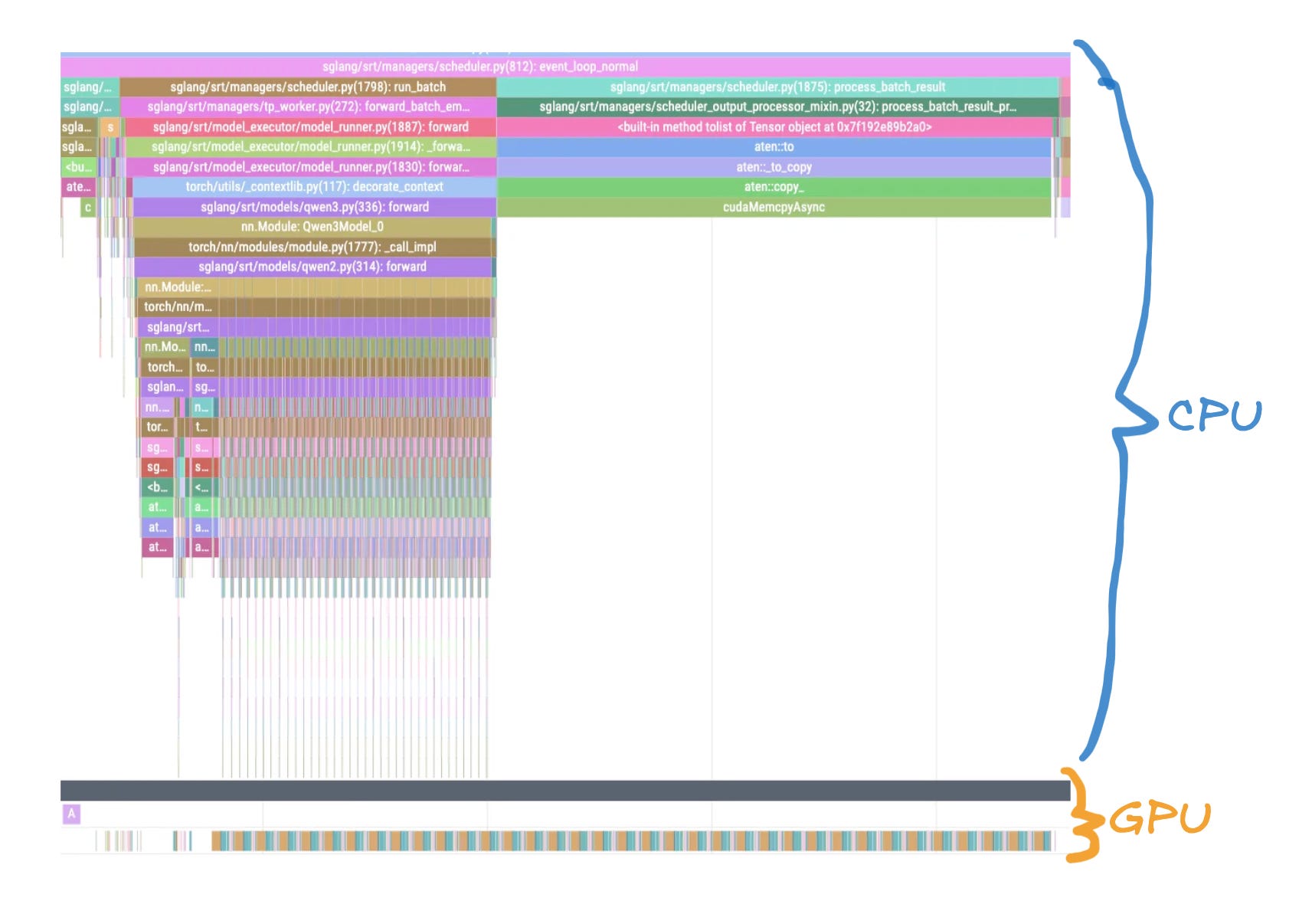
What we calculated while doing the theoretical analysis of the Qwen embedding forward pass, and what we measured via our benchmarking script, can also be observed if we profile the forward pass and look at the individual kernels being invoked. The profile trace can be easily obtained from SGLang by hitting the `start_profile` and `stop_profile` endpoints. All calculations in between these calls will be captured by the torch profiler as demonstrated in Fig. 10.
Before diving into our profiling results, it’s important to understand how to read these traces. Torch Profiler shows both CPU and GPU activity in a unified timeline, but they operate asynchronously.
CPU timeline (top portion): Shows when the host code launches kernels, allocates memory, and performs other CPU operations
GPU timeline (bottom portion): Shows when kernels actually execute on the GPU hardware
Asynchronous execution: When the CPU “launches” a kernel, it doesn’t wait for completion—it immediately continues to the next instruction while the GPU executes the kernel independently
This asynchronous nature means there’s often a visible gap between when a kernel is launched (CPU) and when it actually runs (GPU). When we look at the high-level (Fig. 11) trace of a forward pass, we can clearly see multiple (36) hidden layers being called. The kernels are pretty well packed together.
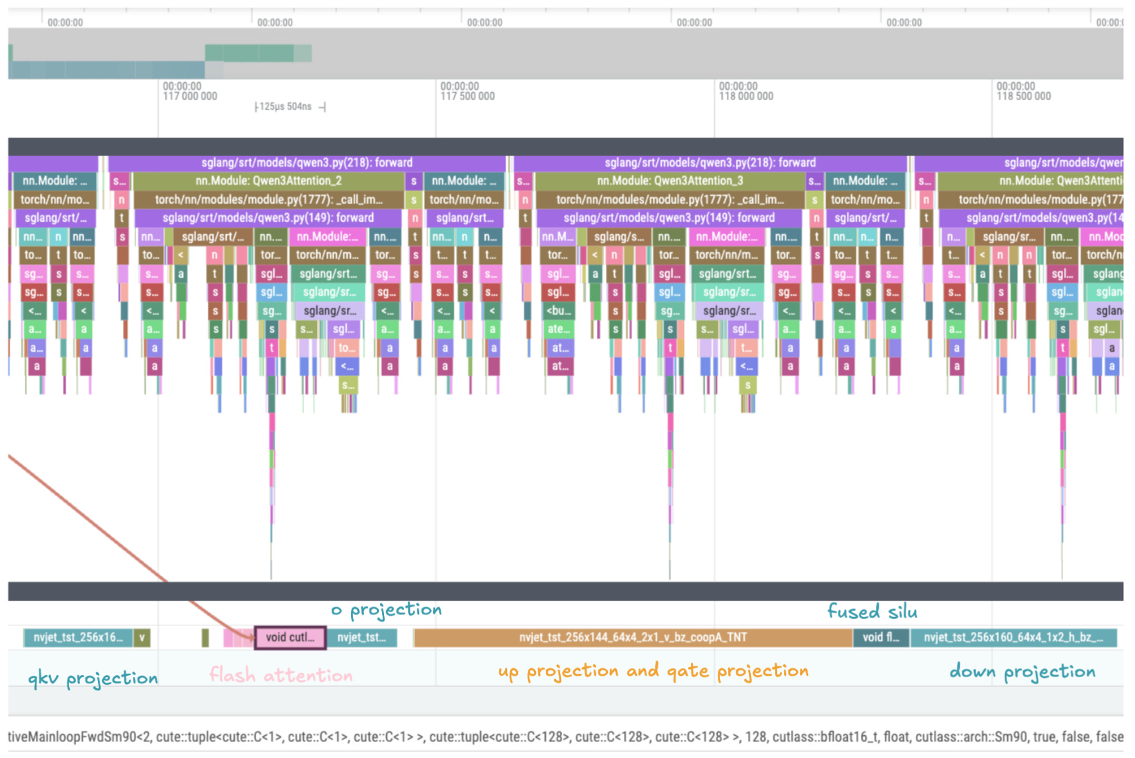
When we look at the single-layer level (see Fig. 12), we can identify the individual components of a transformer layer. Even for a relatively long sequence of 2600 tokens, MLP computation visibly dominates execution time. Additionally, the reader should note that except for the time the GPU is working (kernel) is visible, there are some small, but still existing, gaps between the kernels and kernels invoked to prepare the data (the small pink rectangles before the flash attention kernel). All of these gaps and small kernels add extra overhead to our computation.
When we aggregate all of the kernels invoked during the forward pass, an interesting pattern emerges (see Fig. 13). The majority of time during a forward pass is spent computing nvjet_tst_256x144_64x4… kernels - CUDA highly optimized matrix multiplication kernels. This is another one of the key observations we hope the reader takes out of reading this text. The vast majority of forward passes while calculating the embeddings are spent in matrix multiplication kernels. What it implies is that the 750 TFLOPs we calculated for matrix multiplication in the previous section will be a pretty good proxy for estimating our time of a forward pass, and as a result, the throughput.
Other kernels like fused SILU and RMS norm (primarily from FlashInfer) contribute smaller percentages of wall time and aren't explored further here.
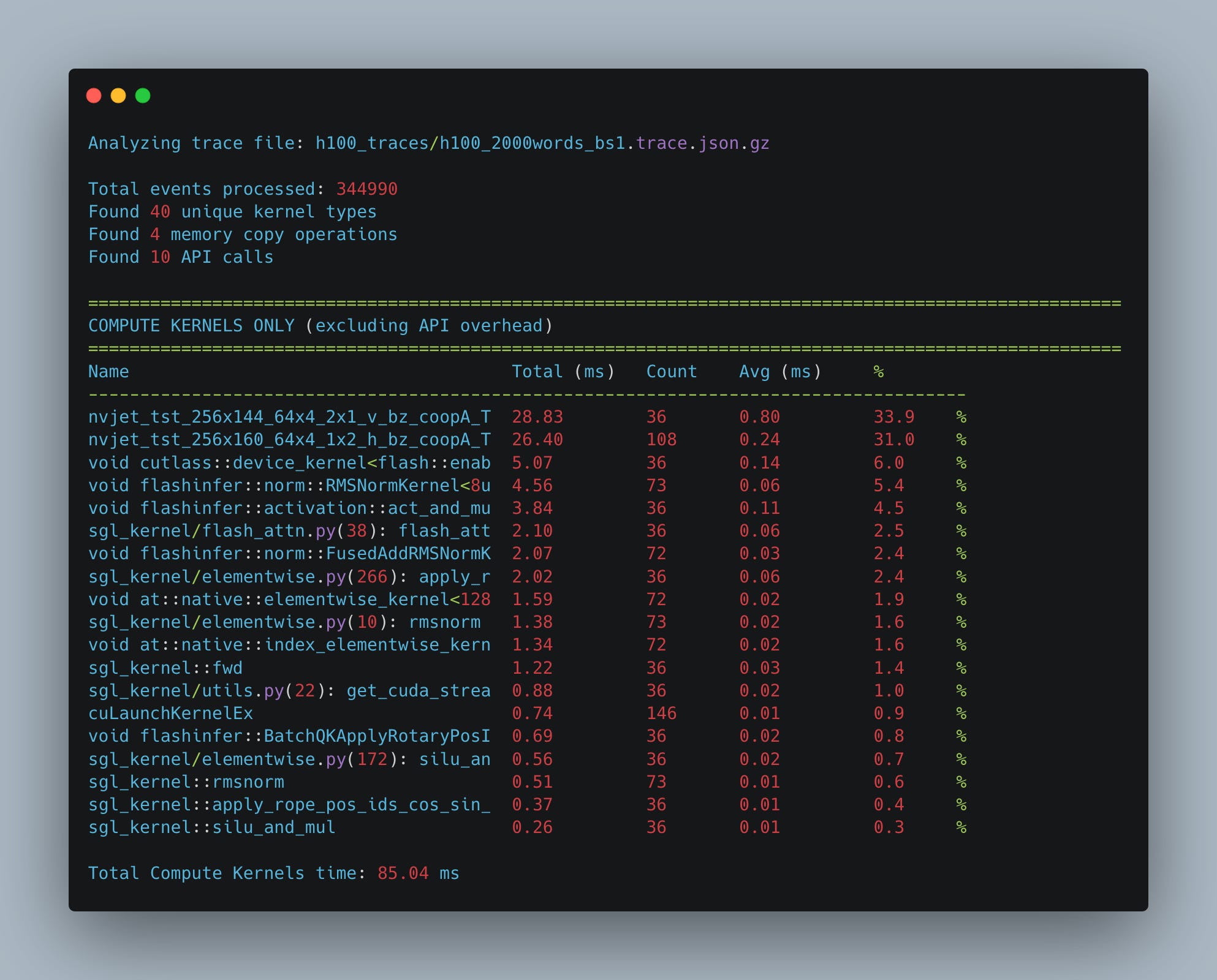
What should be pretty interesting to the reader is how small a percentage of the forward pass is spent calculating the attention. In our 2600-token example, only 6% of execution time occurs in the attention kernel. Note that the flash attention kernel represents just part of the attention block's total cost. As Figure 12 shows, substantial time is spent on QKV projection, O projection, and input preparation (such as applying RoPE).
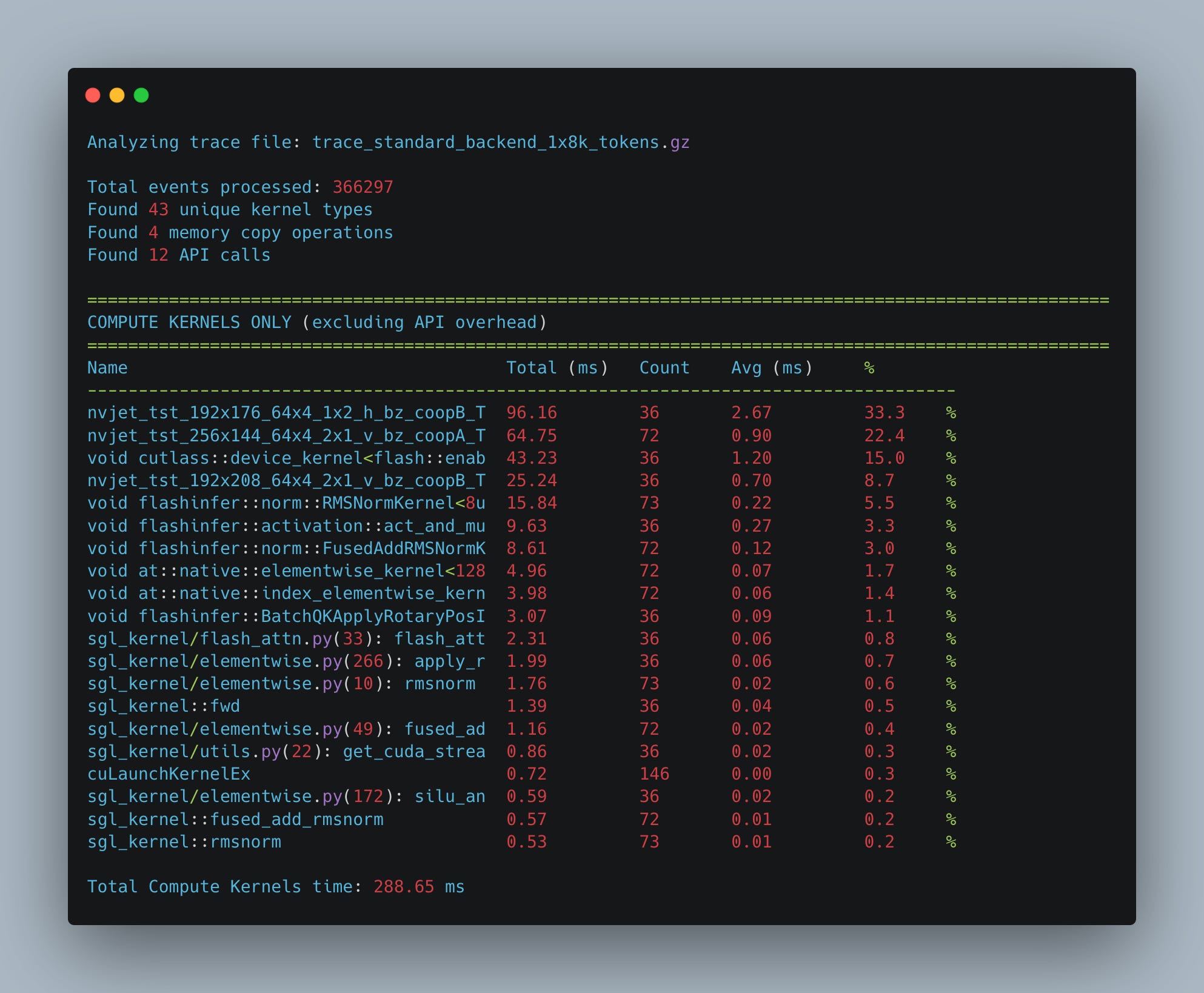
Since attention has O(N^2) complexity with respect to length, and MLP grows linearly (we calculate the up and down projections for each token in the sequence), as we increase the input length, attention will represent a more and more significant portion of the forward pass time. E.g., in Fig. 14 we show that when we increase the sequence length to 8k tokens, the percentage of time spent in calculating the flash attention kernel grows from 6% to 15% of the total time.
When we increase the batch size, the number of operations grows linearly both for the matrix multiplication kernels (we need to handle linearly more tokens) and for the flash attention kernel. You can see (Fig. 15) that as we increase the batch size, the percentage of the wall time remains (roughly) the same.

The traces demonstrate that most time is spent in matrix multiplication kernels. However, the torch profiler only shows that the GPU is working on these kernels—not how efficiently it's utilizing available compute resources. While we might assume NVIDIA's highly optimized kernels achieve good utilization, it would be nice to confirm this.
What we can do is we can run the NCU profile while producing an embedding. Such an option is also available in SGLang, though it is slightly more challenging to make it run than in the case of the torch profiler.
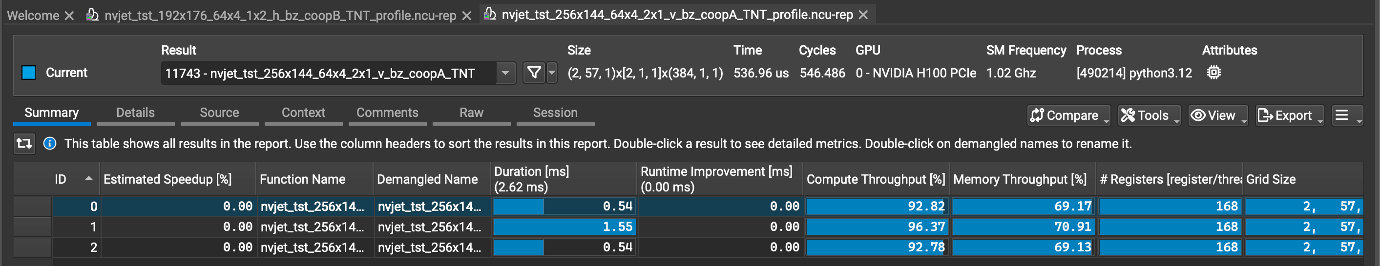
When profiling the kernel with NCU, it becomes pretty evident that we achieve very, very high compute utilization (see Fig. 16). Our compute throughput is pretty close to 100% of utilization. Note how since the majority of time is spent computing, the memory remains underutilized.
Since most of our time is spent in these matrix multiplication kernels, and they by default present a very good compute utilization, this bears the question, “What could be further improved?”
From FLOPs to dollars
As we calculated in the beginning of this text, generating embeddings is incredibly cheap. Embedding an entire English Wikipedia will set a user back around $650. Our contention is that the cheap prices offered to consumers are a result of the underlying cost structure - that producing the tokens is just incredibly efficient and that, due to competitive pressure, the cost savings are passed onto the consumers, driving the price basically to zero.
Based on the experiments we captured in Fig. 7, we can quite easily calculate what the total number of tokens processed per second is at different batch sizes at:
For example, with 1040-token sequences at batch size 4:
In Tab. 1 we present the number of tokens processed each second based on the numbers presented in Fig. 7. What the reader should note is that the numbers saturate around ~45k tokens/s, which once again shows our calculation getting compute bound.
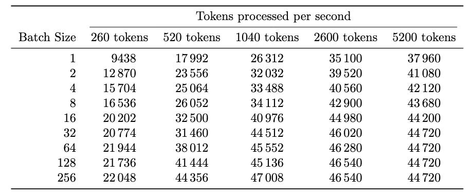
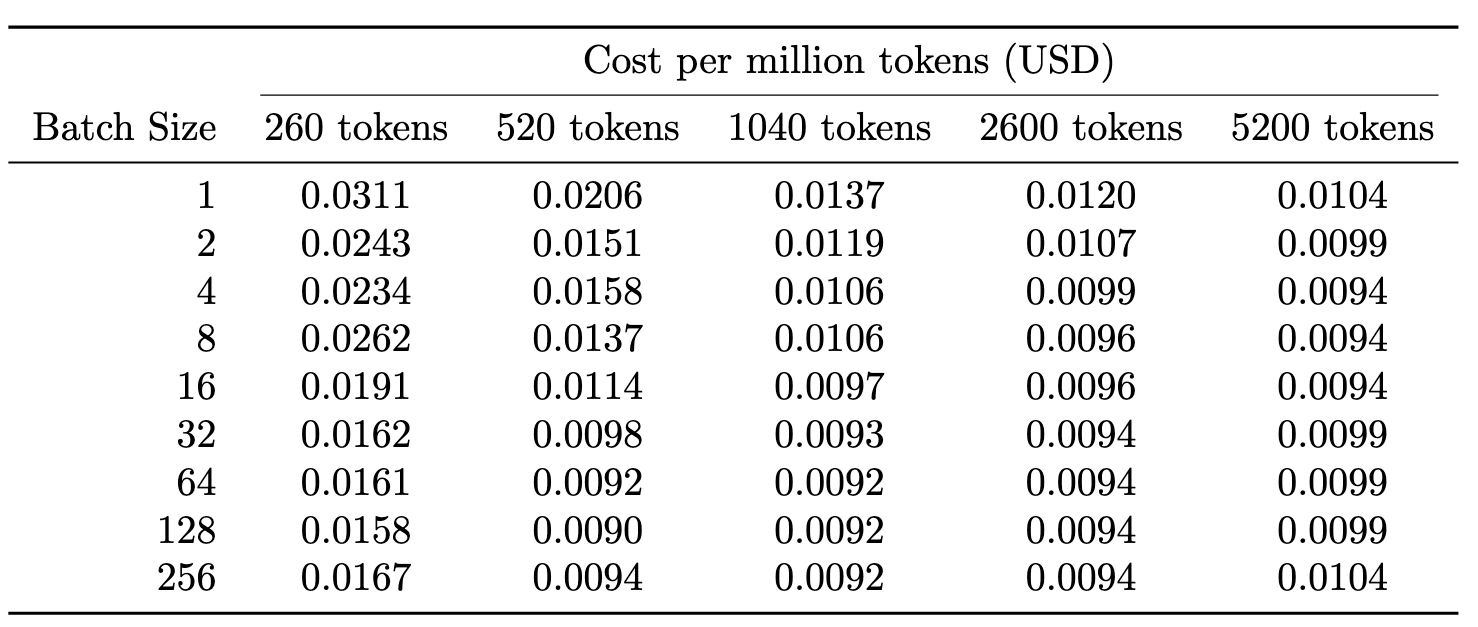
Assuming that we are renting H100 for $2/h, we can estimate the cost of producing a million tokens as:
e.g., for embeddings of an input sequence of 1040 tokens at batch size 4, we calculated above it would translate to around
or 1.66 cents for processing a million tokens.
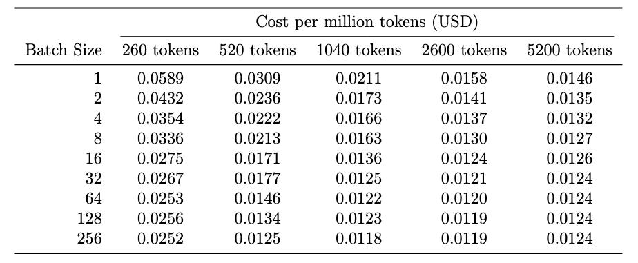
In Tab. 2 we present the estimated pricing for different settings.
The prices estimated above build on the assumption that we enjoy 100% utilization at the given batch size, meaning that 24/7 we get requests coming in that we can compute and charge the user for. In practice we will for sure get periods of higher traffic when your API is bombarded by the requests and quiet periods, e.g., outside of business hours, when our compute will be mostly idling.
Our exact calculations will depend on these computation patterns, how many users you have per GPU, how much latency your users are willing to accept (see Fig. 8), and how time-concentrated our requests are.
Assuming that our typical request will be similar to batch size 4 of a request of size 1040 tokens coming at the same time and this will happen around 10% of the time throughout the day, this would result in 32.2 x 3600 x 24 x 0.1 ≈ 276k requests. In such a case our cost for processing 1M input tokens would be around $0.0166 x 10 = $0.16, or 16 cents/1M tokens. Slightly above the OAI pricing for ada-embeddings.
Other than bringing in more users, could we do anything else to improve our cost structure?
Our metric - FLOPS per dollar
Consider embedding generation from first principles. Our computation pattern has four key characteristics:
We do just a single forward pass.
Our model is in bf16. It is relatively small, occupying only 15.2 GB of space (plus some space for activations); we can easily fit it on a single GPU, and we don’t need high communication between the GPU.
The forward pass is mostly compute bound - having fast memory brings us little benefit.
We know that our most important metric is how fast the GPU can do large matrix multiplications - FLOPS
Since we're primarily FLOPS-bound, the metric we should optimize is FLOPS/dollar. Why pay premium prices for H100's 80GB of memory, ultra-fast memory bandwidth, and high-speed interconnects when our small model doesn't require these features? Most of our time is spent computing, not moving data.
The logical approach is finding GPUs with superior FLOPS/dollar ratios. Table 3 compares three popular options using on-demand cloud pricing: H100 SXM, A100, and RTX 4090.
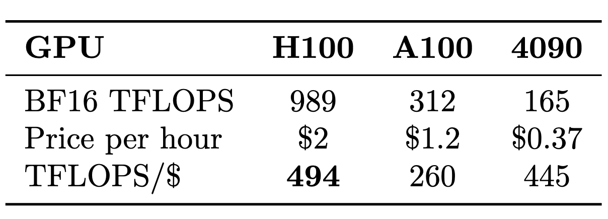
On paper, the H100 dominates this comparison, achieving the best FLOPS/dollar ratio out of the three compared GPUs.5. However, as we showed in Fig. 5, in practice H100s gets power-bound. The 989 989TFLOPS promised by Nvidia are unattainable.
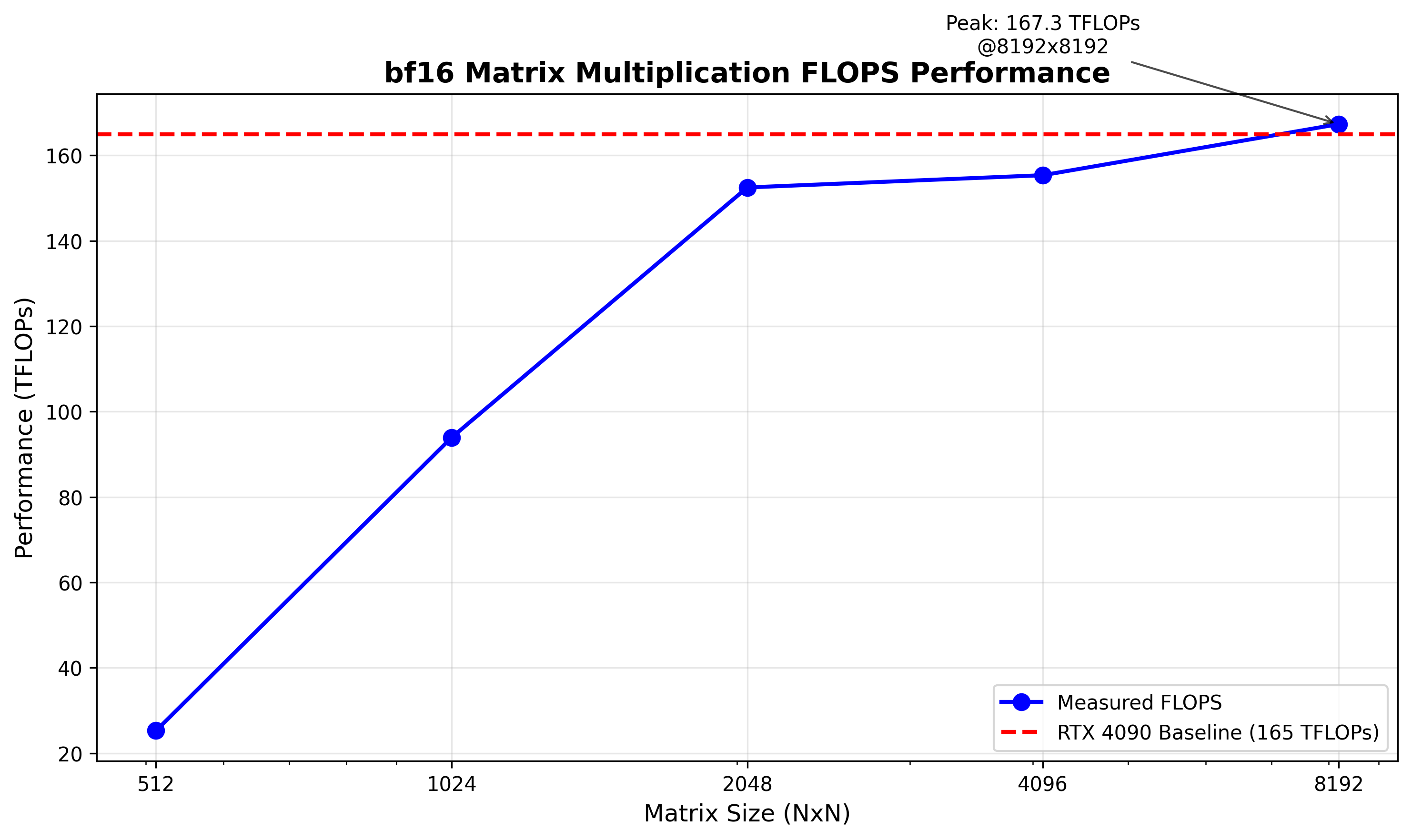
Using the more more realistic 750 TFLOPS (as estimated in Fig. 5), the TFLOPS/$ ratio would drop to 750/2=375, considerably below the RTX 4090's theoretical 445. To verify whether the RTX 4090 can achieve its declared 165 TFLOPS, we ran identical matrix multiplication benchmarks (Fig. 17). The RTX 4090 closely matches NVIDIA's specifications.
The price difference is significant: H100 costs 5.4x more than RTX 4090 ($2/$0.37), while the performance difference is only:
This suggests RTX 4090 should deliver better performance per dollar for embedding generation. Since embedding computation is dominated by large-scale matrix multiplication, this benchmark performance difference should accurately predict real-world embedding throughput differences.
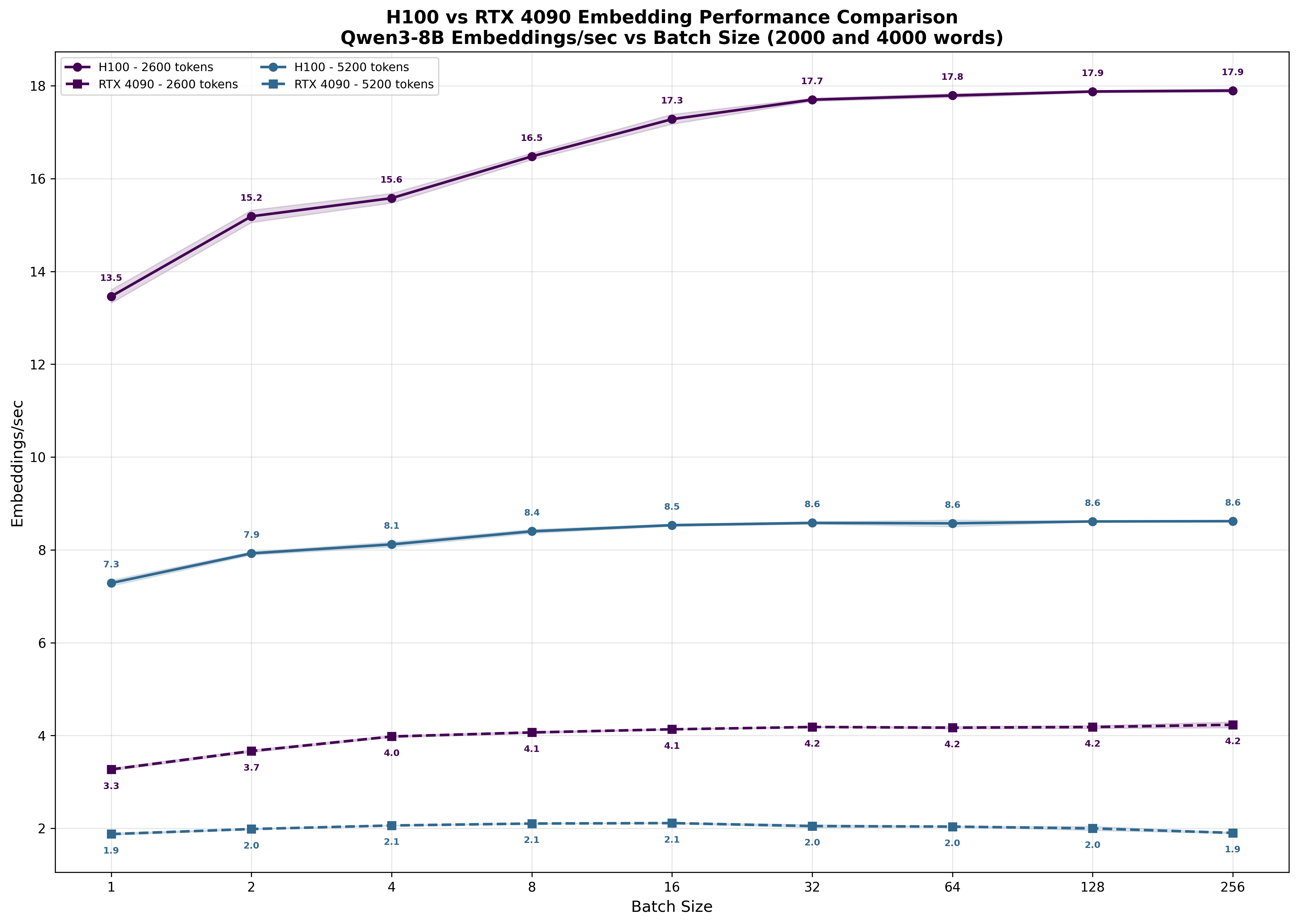
To confirm this prediction, we ran identical benchmarks on the RTX 4090 (Figs. 18-19).6.
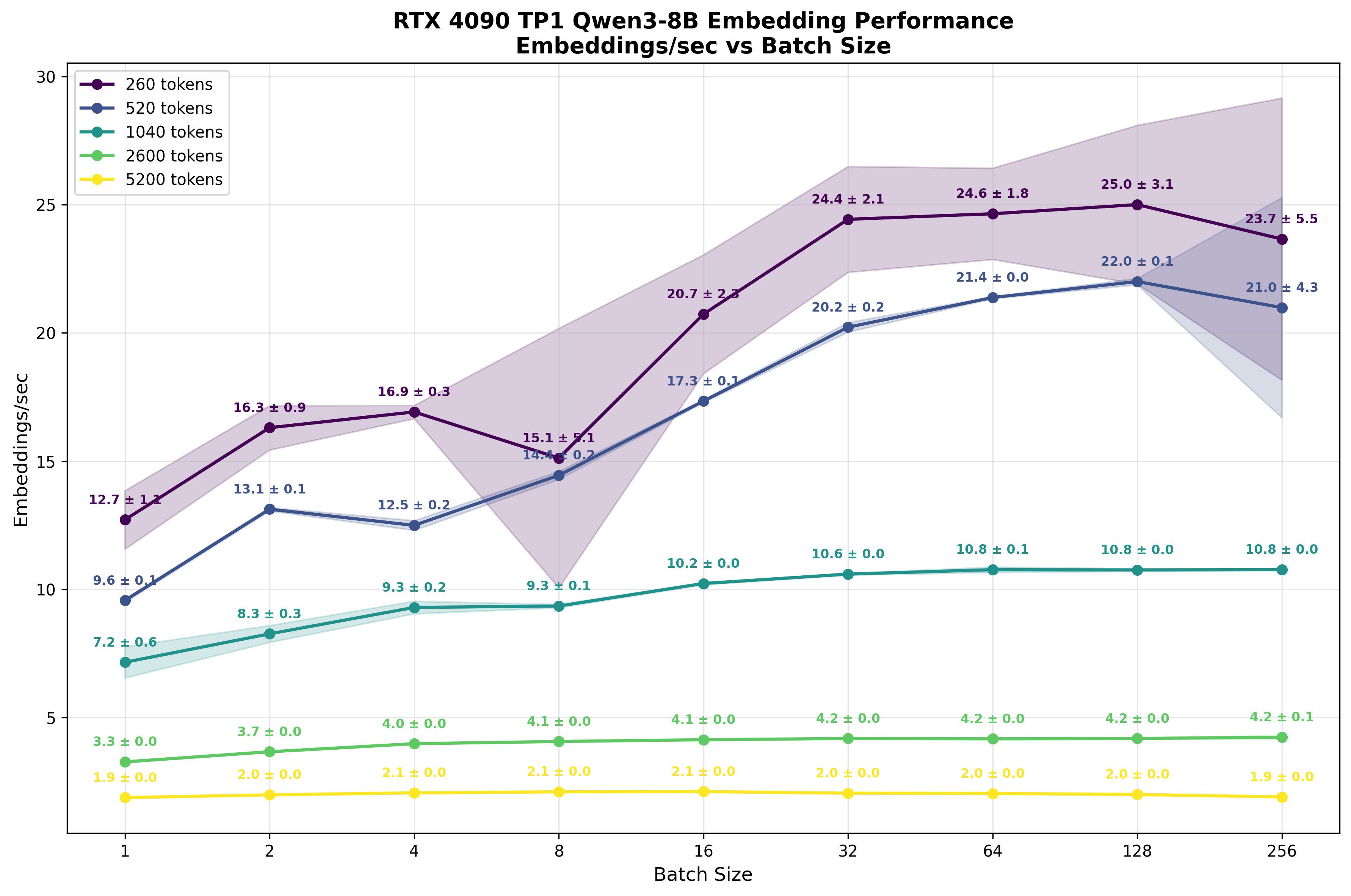
The results mirror our H100 observations: as batch size increases, per-user latency grows (Fig. 19). The RTX 4090 demonstrates the same compute-bound behavior - limited throughput scaling with larger batches but severe latency penalties for individual users.
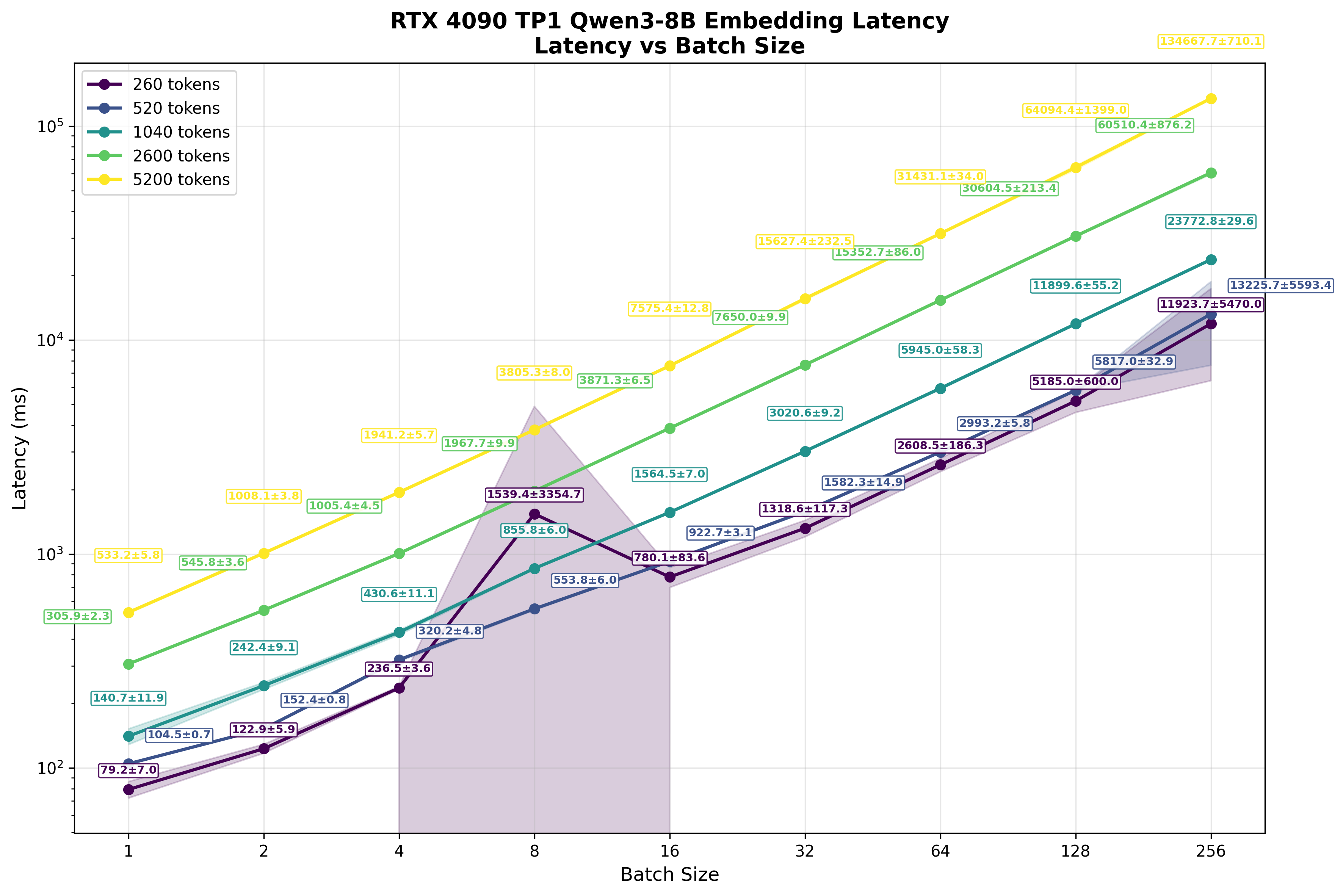
Especially for the shorter inputs, the 4090 performs surprisingly well. The H100-to-4090 performance ratio ranges from 25.3/7.2 = 3.5x at batch size 1 to 45.2/10.8 = 4.2x at larger batches - smaller gaps than the 4.5x difference we measured in pure matrix multiplication benchmarks.
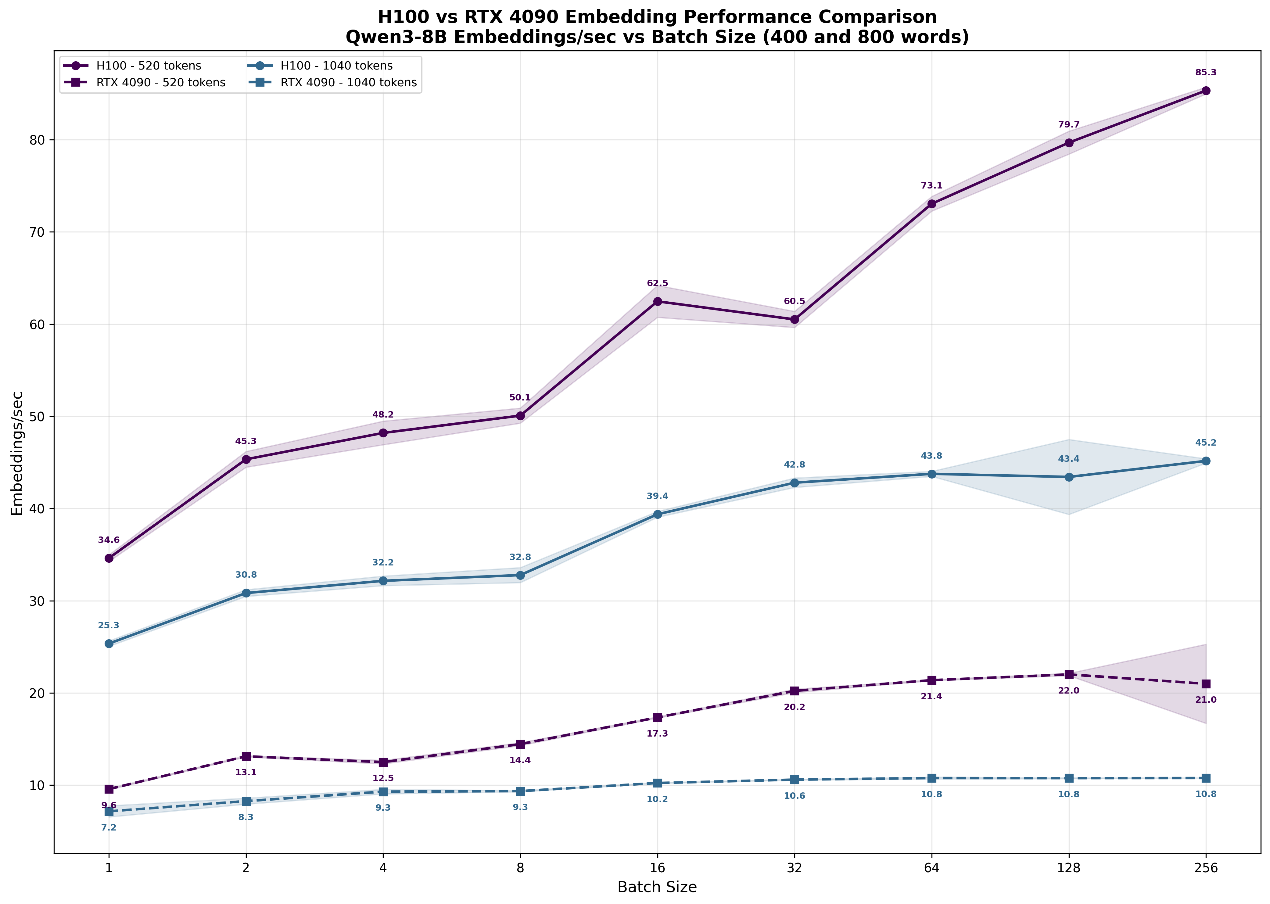
As sequence length increases and we process larger matrices that more fully saturate compute resources, the performance ratio approaches our measured 4.5x matrix multiplication difference.
What should be pretty apparent is that the performance difference is smaller than the price difference between the H100 and the 4090 - meaning that the per dollar spent, we should be able to produce more tokens. To confirm this, similarly to what we did for H100 in Tab. 1, we calculate the number of tokens processed within a second by 4090 in Tab. 4:
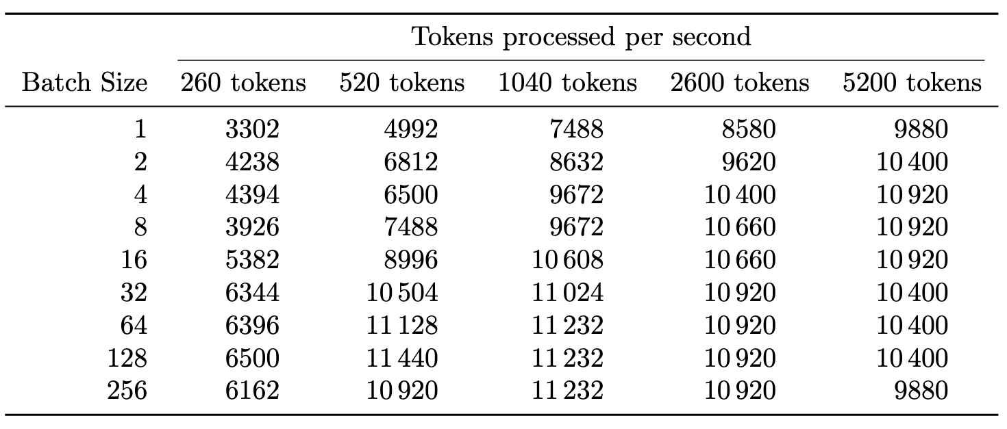
Assuming we pay $0.37 for an hour of 4090 and we use it to continuously embed an input sequence of 1040 tokens at batch size=4, it would translate to around
or around 1¢ for 1M tokens - 36% cheaper than the number we achieved for H100.
In Tab. 5, we present the estimated pricing for processing 1M input tokens. Once again, please note that this assumes 100% utilization; in practice, you won’t be able to process it so cheaply unless you have some sort of a batching system and massive, not time-sensitive demand that can be spread evenly throughout the day.
Note how Tab. 5 demonstrates our point. We were able to find a GPU that offers a superior FLOPS/dollar compared to an H100; this better performance is clearly reflected in the cost for processing 1M tokens. In 4090, in a lot of cases, we are able to drive the price of 1M tokens below 1¢. If we have more demand, we can simply scale the number of 4090s, which should be cheaper than switching to an H100.
Interestingly, for a 4090 that costs only 24x$0.37=$8.8 per day to rent, assuming we continuously get batches of 1040 tokens at batch size=32, it can process
We find it quite remarkable that a consumer-grade GPU that you can rent for less than $9 per day can process 1B tokens a day if provided enough demand.
Noteworthy embeddings are not the only application where you might benefit from prioritizing FLOPS/dollar spent. Prefill, especially in agentic tasks with long context consisting of long tool calls, is another example. Recently NVIDIA released Rubin CPX exactly for this purpose - a chip that’s heavy on compute but light on memory bandwidth, using cheaper GDDR7 instead of expensive HBM. It’s the same logic we’ve been discussing: when you’re compute-bound, optimize for FLOPS per dollar.
Summary
We started this text mentioning that embedding APIs are very cheap to use, and we argued that this underlying price is derived from low costs of producing the embedding representations rather than being subsidized below the cost of production.
We took the leading open-source embedding model, Qwen3 8B Embedding, and analyzed it in detail, including theoretical estimation of the FLOPS and real-world performance benchmarking. We did a deep dive into what is happening under the hood, showed which kernels are invoked, and showed how the majority of the execution time is spent in large-scale matrix multiplication.
Lastly, based on the observed performance, we calculated the price for processing 1M input tokens for different input-tokens/batch-size setups. Please once again note that the numbers shown assume a situation in which you enjoy 100% utilization, with the request being continuously batched.
GPUs are incredibly efficient at these sorts of workloads, driving the price down to zero. Since all leading models converge on a similar latent representation, and perform comparably no one has a pricing power enabling them to command higher prices. As the model gets more efficient, compute and energy get cheaper, and this situation will move towards the generative models as well. The embedding situation offers a nice pre-taste of the "intelligence involution” that is coming …
Acknowledgments
Thanks to Johannes from Prime Intellect for providing me with the compute to run these experiments, and to Jo (check out his new retrieval company), Felix, Pablo and Szymon for giving me comments for parts of this text.
@online{tensoreconomics2025embeddings,
  author = {Piotr Mazurek},
  title = {Why are embeddings so cheap?},
  url = {https://www.tensoreconomics.com/p/why-are-embeddings-so-cheap},
  urldate = {2025-09-24},
  year = {2025},
  month = {September},
  publisher = {Substack}
}Prices as of 8.09.2025
Before each experiment we do a quick warmup of the GPU. We also repeat each experiment setup multiple times (e.g., 10) and measure the mean and the variance.
We have a small difference between the estimation and experiment. In our estimate we use 1024 tokens; in experiments we use 1040 tokens—a ~1.5% difference. It has a negligible impact on the calculations; we just want the reader to know we are aware of this minor difference.
There is some limit to this; as we increase the batch size, the KV cache will represent a more and more substantial portion of the total memory loaded. As the KV cache starts to dominate the load, the per-user experience will start to be more and more impacted by the batch size.
Note that if you were to buy these GPUs the ratio between the devices would be different, e.g. a new 4090 can be aquired for ~$3200 while a brand new H100 SXM5 would cost around 10x more.
We rented a 4090 on RunPod, running within a container.