AI infrastructure in the "Era of experience"
Intelligence involution, economies of scale in RL, everything async and multi-turn.
In the famous essay from May 2025, “Welcome to the Era of Experience,” Rich Sutton and David Silver proposed a new paradigm of training AI models - models that learn not through predicting the next word against text scraped from Common Crawl, but through gaining experience via interaction with environments. As we approach the exhaustion of easily scrapable text data, we predict we’ll observe a shift toward AI models increasingly trained in this fashion via reinforcement learning (RL). In this text, we discuss the technical details underpinning this process.
The text proceeds as follows: First, we introduce the concept of intelligence involution and discuss its consequences and why there is currently a strong incentive for custom RL models; then, we explain the basic principles behind GRPO; we briefly explain why RL training is so information sparse; and we do a deep dive into LoRA and the compute advantages of training and inference it unlocks. Then in the last section we discuss the broader implications; we show how the tech foundation can enable the emergence of the reinforcement fine-tuning (RFT) industry; we highlight where economies of scale can be realized and what some potential first applications of custom models are. We mention the remaining open challenges and the fundamental limitations that can potentially make RFT a similar flop as the first wave of SFT has been.
We intend this text to provide the reader with the theoretical basis needed to reason about AI infrastructure in the context of reinforcement learning. We argue that in the next 6-12 months there are significant opportunities for new businesses to be built around recent developments in RL, particularly for product companies to build sustainable moats through custom models trained on their proprietary environments, as well as for infrastructure players to build “picks and shovels” enabling the RL economy.
Intelligence involution and its consequences
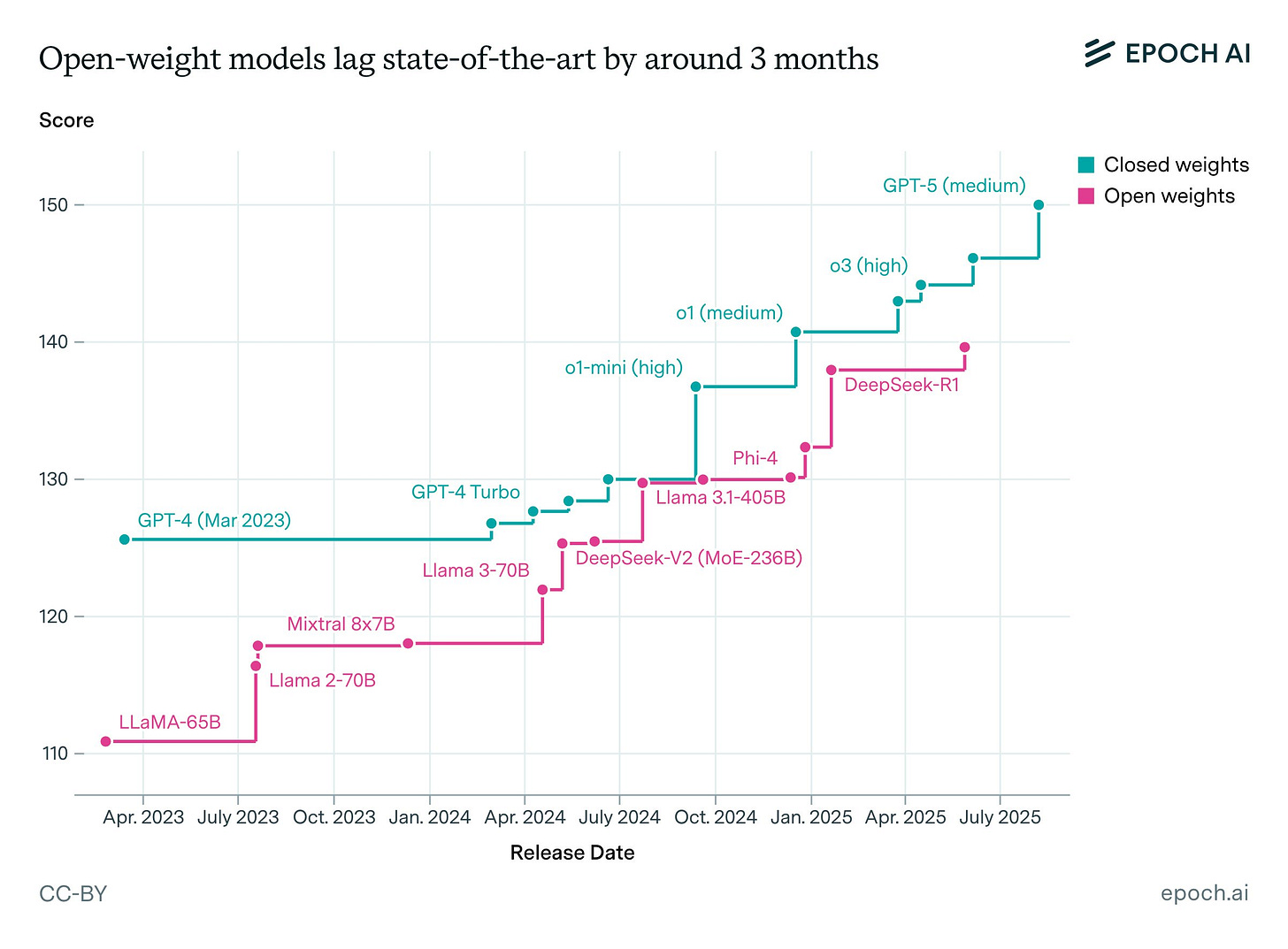
As of late 2025, it appears that the gap between available LLMs is extremely small. There are marginal differences between proprietary LLMs, with some models slightly stronger in some niches like creative writing or coding, but overall differences seem to be diminishing over time. Moreover, the gap between open-source and proprietary models is rapidly closing. EpochAI estimates (see Fig. 1) the lag at around three months; with Kimi K2 Thinking’s release, some argue the gap has largely closed1.
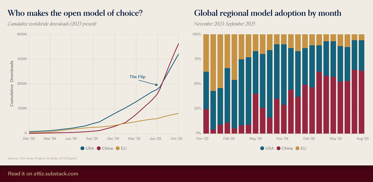
Interestingly, China now leads open-source development. Chinese models have overtaken Western ones in cumulative downloads worldwide (see Fig. 2). While downloads aren’t a perfect proxy for popularity2, the Twitter “vibe check” seems to confirm this. These days, every RL experiment appears built on Qwen. Recently, Cursor and Windsurf appear to have built their models on top of Chinese foundations as well.
There are dozens of Chinese labs in this space, and it seems like every week a Chinese food delivery company or consumer electronics firm releases a competitive AI model. Next-token prediction appears to share characteristics with EVs, solar panels, or batteries - where Chinese “capital markets” are capable of supporting dozens of entities that relentlessly compete with each other, continuously driving down the price per unit of intelligence, glutting international markets, and making it close to impossible for competitors abroad to make any revenue with models not at the absolute bleeding edge3. While OpenAI, Anthropic and Google remain ahead and this doesn’t yet apply to them, if the trend continues, it seems inevitable their margins will eventually be affected.
We refer to this phenomenon as intelligence involution, where - similar to EVs or solar - competition is so fierce that everyone makes close to zero profits, moats only come from scale, and the pace of competition slowly bleeds out anyone not at the absolute frontier.
Since competition is so fierce, it continuously drives down the price of tokens. For example, DeepSeek during the transition from v3 to v3.2 dropped prices from $2.19 to $0.42 per million output tokens - 5x cost reduction in a span of a few months while simultaneously boosting general model capabilities.
With competition in general-purpose models this brutal, requiring absolute frontier performance to generate any substantial revenue, the obvious choice for less sophisticated players seeking quick profits is model specialization: targeting a niche that should be more defensible than competing in the foundation model space.
Traditionally, companies specialized foundation models through Supervised Fine-Tuning (SFT). The approach was straightforward: collect input-output pairs for your domain, then retrain the model to mimic those outputs. However, as we enter the era of reasoning, SFT is being squeezed out of relevance by a “pincer movement” - it is becoming economically irrational for simple tasks and technically insufficient for complex ones.
For static knowledge or stylistic specialization, SFT has become largely unnecessary. Modern base models are now powerful enough that in-context examples (few-shot prompting) match fine-tuned performance without the complexity of managing model weights.
With the commoditization of prompt caching, this approach is also much cheaper. As of late 2025, caching allows us to “pin” massive instructions into memory at near-zero cost. For example, as of November 2025, DeepSeek charges $0.028 per million cached tokens. Storing 10,000 tokens of examples in the prompt and serving 1 million requests costs just $280 in caching fees:
This is potentially cheap enough to eliminate the need for SFT entirely for straightforward tasks. Fine-tuning a custom model for the same task would cost thousands in compute and engineering time, only to yield a model that becomes obsolete the moment a better base model is released.
While caching kills SFT at the low end, the “Reasoning Data Barrier” kills it at the high end. Even if human data were available, SFT creates a fundamental ceiling: it limits models to mimicking human baselines rather than discovering novel strategies that surpass them. As per the era of experience, there are certain problems for which prompt-answer pairs simply do not exist. The only way to discover the right reasoning chains or tool sequences is for the model to interact with an external environment and observe the effects of its actions. Based on these observations, the model’s behavior is adjusted iteratively. Critically, we explicitly assume the correct steps are unknown upfront and can only be learned through interaction - by observing how the environment responds and adjusting accordingly.
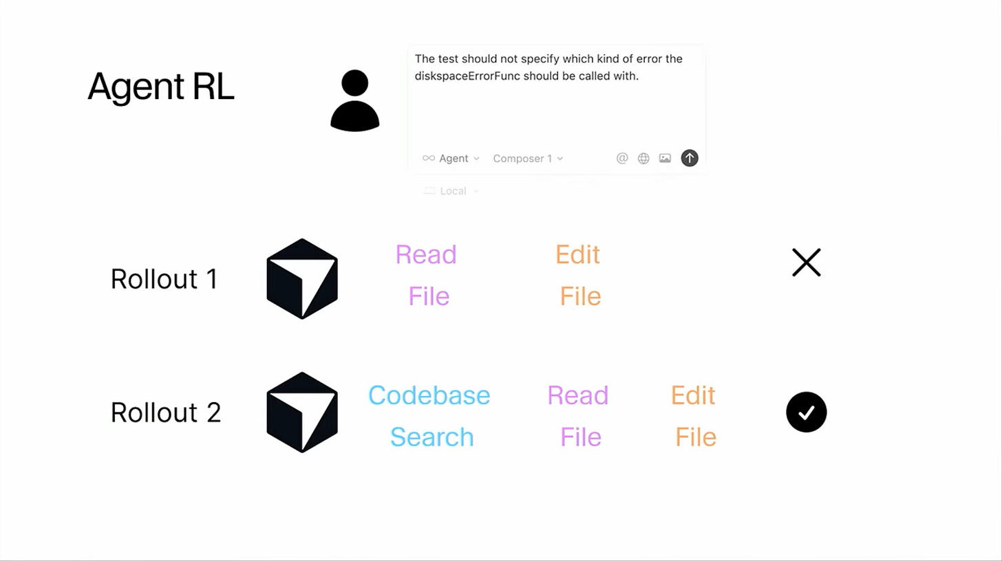
The challenge intensifies with tool-calling and agentic workflows. When models need to orchestrate multiple tools - whether executing Python code, performing web searches, calling APIs like the SharePoint MCP server, or any other programmatic action (see Fig. 3) - the correct sequence of tool invocations and their specific parameters must be discovered through trial and error. Manually creating training examples for every possible toolchain and edge case quickly becomes infeasible.
This creates a natural opening for custom models. Many companies would prefer to own their intelligence stack entirely - for data privacy, cost control, and because they don’t want to depend on vendors whose priorities and pricing might shift unpredictably. Previously, this wasn’t feasible: building competitive models required frontier-level base intelligence that only a handful of labs had.
Intelligence involution changes this calculus fundamentally. With open-source models now matching proprietary performance at a fraction of the cost, companies can build defensible RL-specialized models on top of these commodity foundations. The moat comes not from superior base intelligence - which is rapidly commoditizing - but from proprietary access to specialized environments and the continuous learning loops within them. These environments are unique and proprietary: a company’s internal research infrastructure spanning SharePoint, Confluence, and legacy enterprise systems; an e-commerce platform’s feedback loop where model behavior is continuously refined based on observed customer actions; a SaaS product’s onboarding flow that adapts based on real user engagement patterns, etc. None of these can be replicated by GPT-5 simply because OpenAI never had access to these interactions during training.
However, this defensibility comes at a cost of scale. Training a model for a specific environment to solve a specific problem is inherently less scalable than a single base model like the one powering ChatGPT, where hundreds of millions of users interact with the same foundation model, controlled purely through prompting.
To understand the cost structure and opportunities in RL, we need to examine how these models are actually trained. This requires introducing a few key concepts: GRPO, LoRA, and the fundamental information-theoretic principles that make RL feasible at scale.
GRPO 101
The “renaissance” of RL for large language models (LLMs) can be traced back to the introduction of Group Relative Policy Optimization (GRPO) in DeepSeekMath: Pushing the Limits of Mathematical Reasoning in Open Language Models in April 2024. GRPO was the fundamental technique that enormously simplified running reinforcement learning with verifiable rewards (RLVR)-type training. Later it was applied in the famous DeepSeek R1 model that shook the global financial markets in January 2025.
The GRPO algorithm is conceptually quite simple; it can be compressed to 12 lines of pseudo-code (see Fig. 4). The main innovation comes from the fact that, in contrast to previous RL methods like PPO, it is far simpler to implement. There is no need to train a separate critic model, and as measured empirically, it proves to be much more stable and sample efficient.
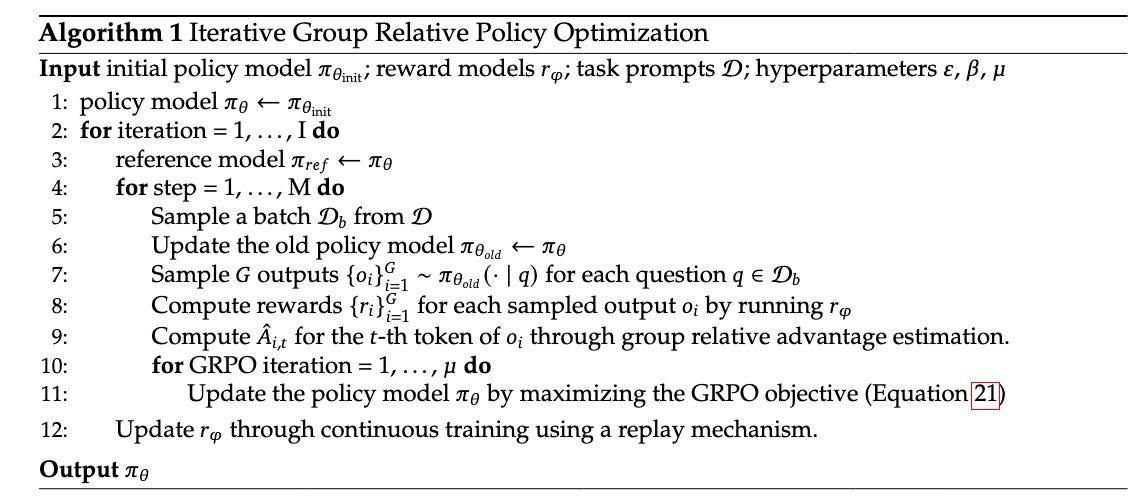
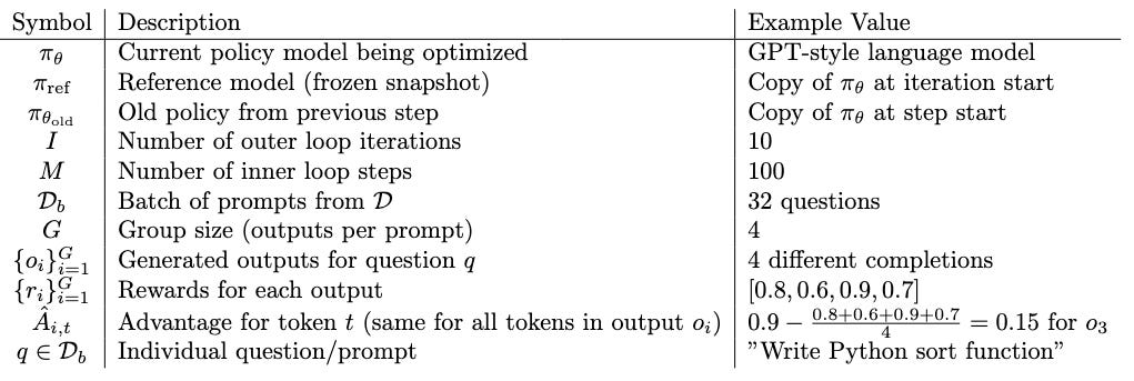
While it might seem complicated at first glance if the reader is unfamiliar with RL notation, upon closer inspection it is pretty simple. In Tab. 1 we present a detailed explanation and example values for all symbols in the algorithm from Fig. 4.
GRPO is an example of so called gradient policy optimization algorithm. We use this name to refer to reinforcement learning methods that directly adjust a policy’s (model`s) parameters using gradients to maximize expected cumulative rewards. In gradient policy optimization algorithm we traditionally have two phases:
Rollout generation: Using the current policy, we generate outputs. For LLMs, a rollout is the sequence of tokens produced for a given prompt (see variable `outputs` in Fig. 5).
Optimization step: We evaluate the generated rollout with a reward signal, then use the gradient of the policy (which shows how to change parameters to increase reward) to adjust the model parameters.
In GRPO, for each prompt we sample G answers, calculate the average reward for this group, and subtract it from each individual reward to get the advantage - hence the name “group relative” policy optimization (see Fig. 5).
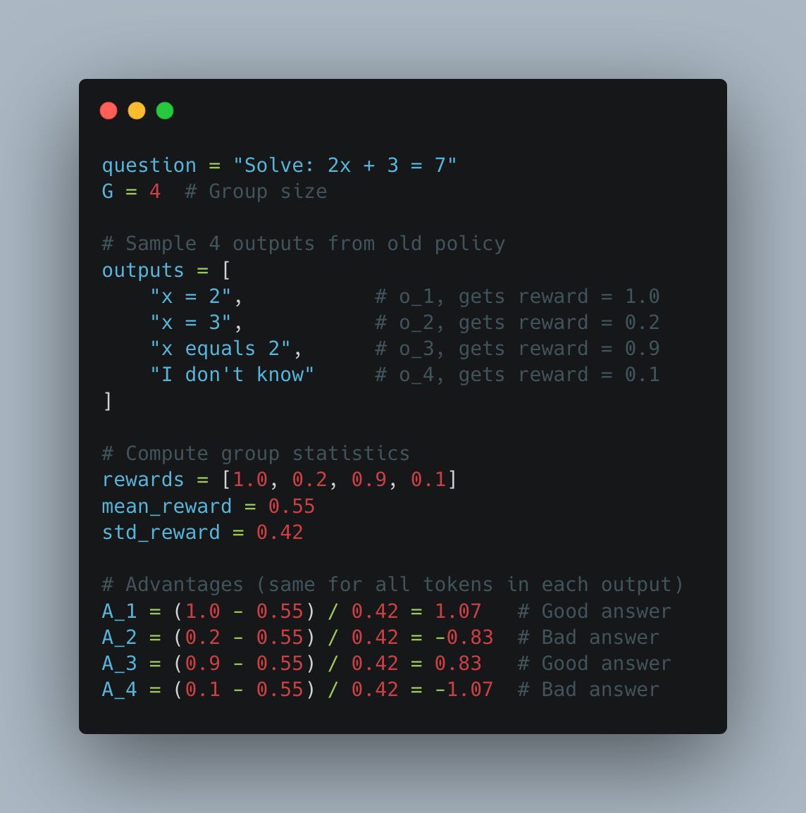
During the training step, we first calculate the ratio of log-probabilities: new policy divided by old policy (see Fig. 6). We apply PPO-style clipping to this ratio, preventing the model from diverging too far from its previous version (previous optimization step). This clipped ratio is then multiplied by the advantage. As shown in Fig. 5, the advantage measures how much better (or worse) each completion performs relative to the group mean, to other completions for this exact prompt.
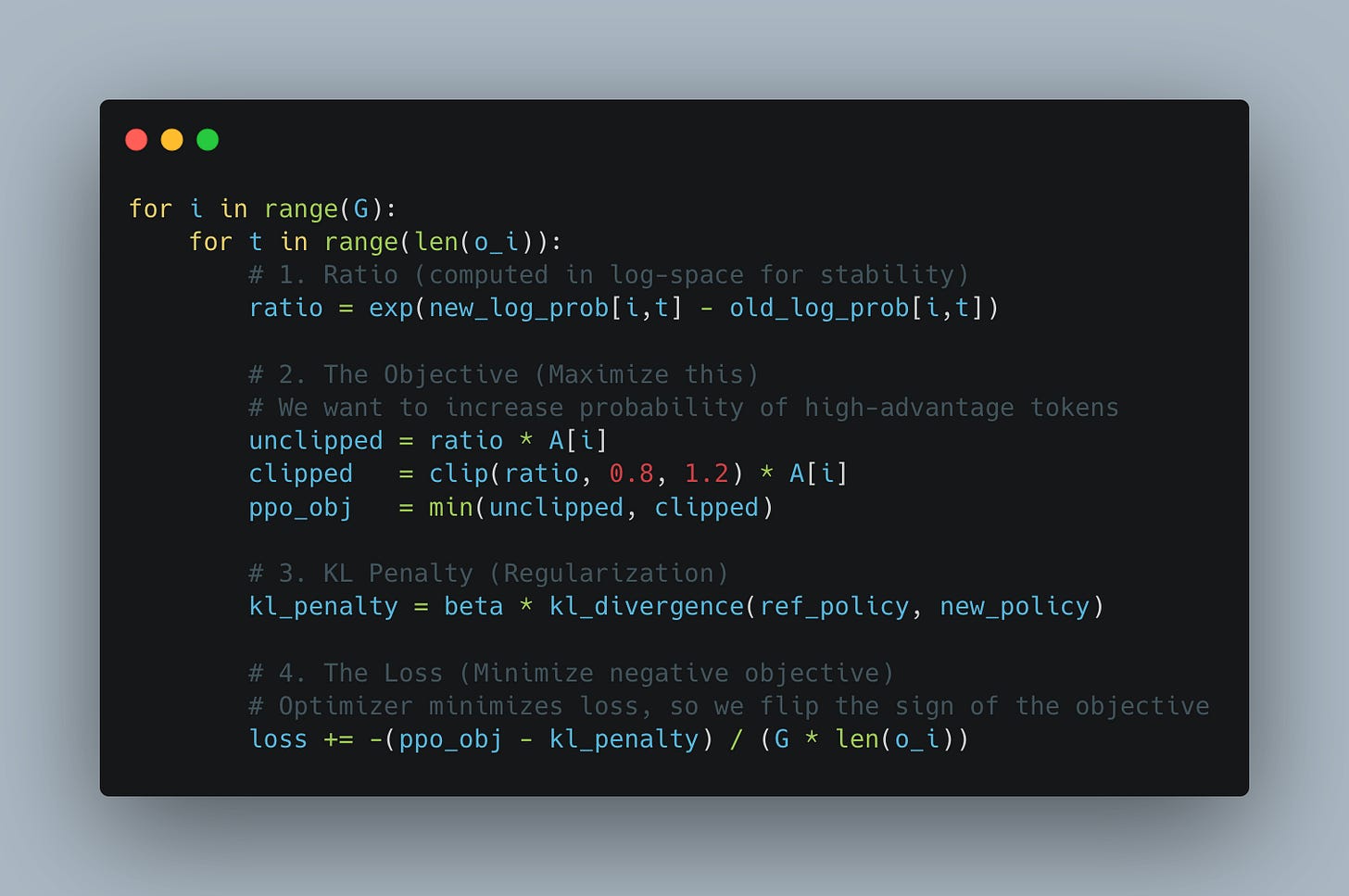
The core idea behind every RL algorithm is to shift the model’s weights, so that high-scoring outputs become more likely and low-scoring ones become less so.
A key limitation specific to GRPO is that, unlike methods with a learned Critic (like PPO), it assigns the same advantage to all tokens in a sequence. While this means equal credit is assigned even in mixed-quality outputs- for example, in a multi-turn WORDLE game where the model guesses incorrectly for three turns but succeeds on the fourth - we accept this approximation because it removes the massive overhead of a value model. In practice, DeepSeek observed that this coarser heuristic is not only significantly cheaper to calculate, but often leads to more stable training dynamics than trying to learn a complex token-level value function.
Just 1 bit per rollout
The “defining” blog-post of the recent boom in RL is “LoRA Without Regret” by John Schulman and the Thinking Machines team. The argument the authors make is that because policy gradient methods (like GRPO) are so information sparse (only 1 bit per rollout) LoRA adapters have enough capacity (enough parameters) to efficiently learn all of this information without the need to modify the original model parameters. This has profound implications for both training and inference which we discuss in detail in the next section.
As the authors put it:
… when we get a few key details right, LoRA learns with the same sample efficiency as FullFT and achieves the same ultimate performance.
The intuition behind this goes as follows. In GRPO, the gradient update for each rollout is proportional to
where q is the prompt, o_i is the generated output (rollout), and A_i is the advantage (reward minus group mean).
The gradient has two components:
Direction
shows how to change the policy to make output o_i more likely. This depends only on the current policy π and the sampled output—it contains zero information about the reward.
Advantage
A_i s the same for all tokens in output o_i. This scalar is where ALL information about the reward function resides.
By the data processing inequality:
and:
where H is entropy (the maximum information content).
While the calculated Advantage is technically a continuous real number (due to normalization against the group mean), its information content is bounded by the granularity of the reward function:
If reward is binary (correct or incorrect)
If we have granular reward - the reward allows for partial credit (e.g., 5 levels: 0,0.25,0.5,0.75,1.0)
Depending on how “granular” your reward is it log_2(N) is the upper bound of what a single rollout provides.
This is much more sparse signal than the supervised training where each token provides ~1 bit of information, so training is way less efficient. It is possible that our rollout generates tens of thousands of tokens, and we put in hundreds of thousands of input tokens the tool calling, and all of this will be summarized into a few bits worth of information, requiring us to run tens of thousands of rollout to learn anything useful.
While this approach is inherently inefficient, as we previously discussed, in cases where we don’t know the correct labels, this “exploratory” approach seems to be the only one we know that works reliably.
The upside of this extreme information sparsity is that it can be efficiently encoded with very few parameters. To quote the Thinking Machines team:
Past work has shown that neural networks can store 2 bits per parameter. These results pertain to the maximum amount of information absorbed in the long-training limit, not to the compute efficiency or rate of learning.
The Thinky team showed (see Fig. 7) that LoRA adapters of fairly low ranks can learn from RL basically as well as full model fine-tuning. These results have since been independently replicated by many people in the community (see Fig. 8).
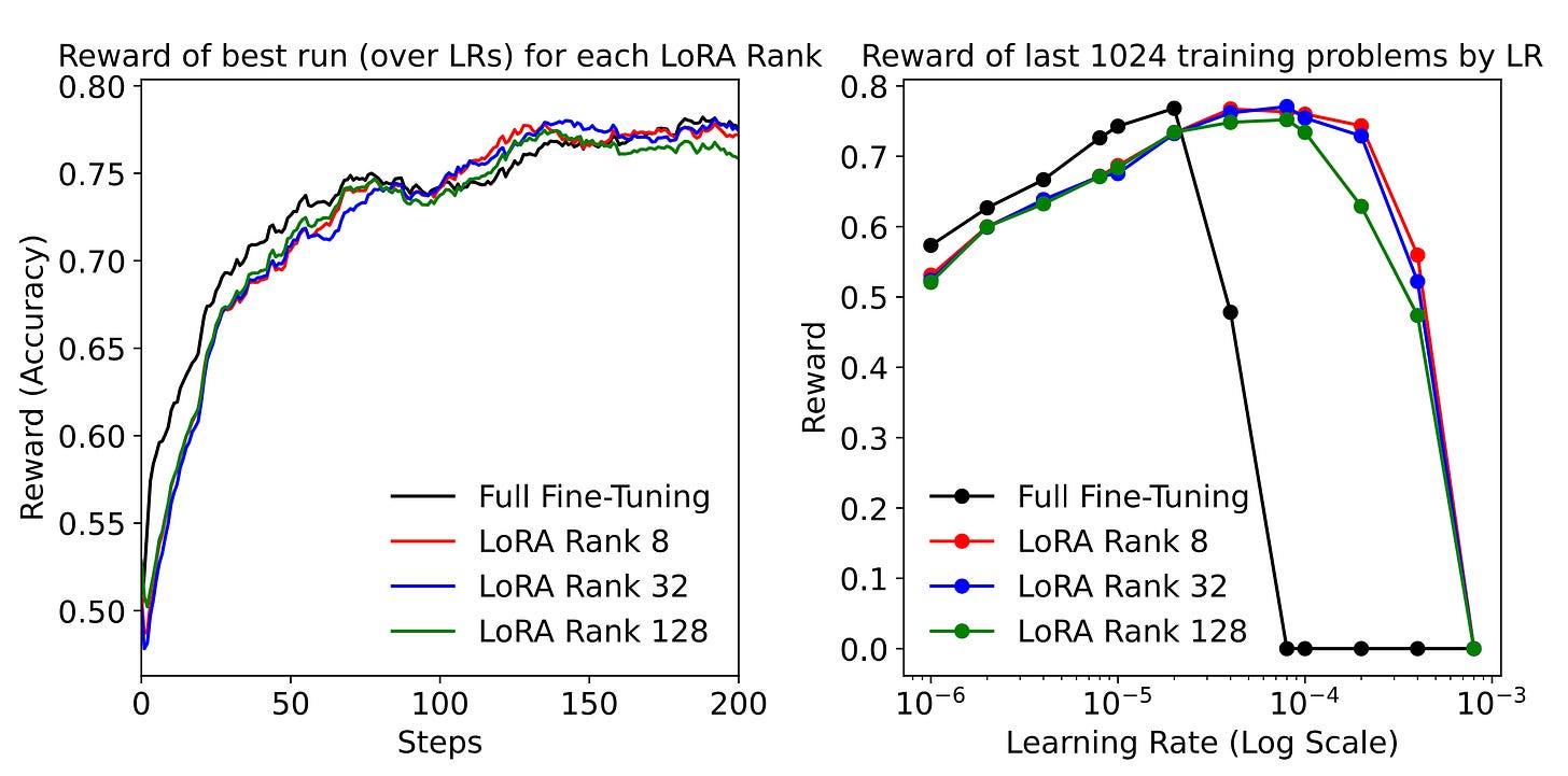
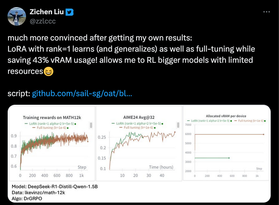
This has profound implications for the economics of training and inference. LoRA makes it possible to train massive models on relatively modest hardware (within a single node), as long as the model parameters fit into memory. Moreover, if the model customization relies on LoRA adapters running on top of a single base model, this has significant effects on the economics of serving such models. It becomes possible to batch together multiple requests from multiple users, use a single base model, and assign different adapters to every request in the batch. This makes inference significantly more affordable. An inference provider might reuse a single base model for thousands of clients, each with their own custom adapter, serving their own custom-trained RL model.
In the next sections, we will delve into the details of why LoRA is so much more efficient in model training and why it has a much smaller memory footprint. We will then explain how multi-tenancy works in a modern inference engine and show how well such models perform and scale. We want to highlight once more the key insight: LoRA fine-tunings perform comparably to full model fine-tuning when trained with policy gradient methods such as GRPO (“no regret”). Because the training signal is so information-sparse, there’s no penalty for training fewer parameters.
Backpropagation and LoRA
Before we proceed to training and inference, we should introduce the two concepts:
How backpropagation in model training works.
How low-rank adaptation (LoRA) works.
Let’s start with backpropagation. Consider a simple 2-layer neural network with sigmoid activation. The forward pass goes as follows:
Now if we intend to train the said network, we need to define some objective we want to minimize (J) and we will minimize it using stochastic gradient descent (SGD). We want to optimize the parameters (weights) of the network to minimize our loss (the objective we defined). To find these values, we use the chain rule.
As a reminder, the chain rule states that for composite functions:
For multiple nested functions, we apply the chain rule repeatedly:
A neural network is exactly this type of composition. Notice how our forward pass creates a chain of functions:
Hence to calculate the gradients we need to run the following steps:
Notice how to calculate the gradient with respect to W2 we need to store the values of intermediate activations - input to the layer 2, a1. This requirement creates a significant memory burden: we must cache these intermediate activations during the forward pass to use them later in the backward pass. Crucially, this cost scales linearly with the batch size. For every additional example we process in parallel, we must allocate memory for its specific activations, explaining why increasing the batch size rapidly consumes available VRAM.
What is also important to notice is how much memory is consumed by storing the gradients of parameters. Since we need a gradient for every single weight in the layer it takes as much memory to store the gradients as it takes to store the weights themselves, further increasing the memory footprint.
In practice, estimating the memory footprint gets even more complicated. Some optimizers require additional memory - Adam, for example, stores momentum and variance estimates for each parameter, often doubling or tripling the memory needed beyond just weights and gradients. Our intention here is to provide the reader with intuitions on where compute and memory costs come from in model training, as this context is crucial for understanding why LoRA makes training more efficient.
Under the hood, for the forward and backward pass, PyTorch implements the interface from Fig. 9. Notice how we need to cache the values of layer inputs (x) and how we need the values of the gradient with respect to the input from the next layer (grad_out) to come as an input parameter.
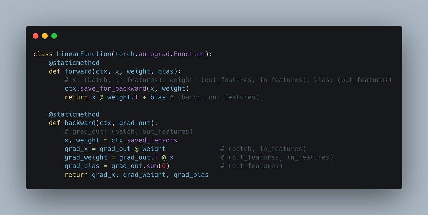
Looking at this, it is quite easy to see how we have to do roughly twice as many operations during the backward pass as we do during the forward. In the forward pass we need to do a single matrix multiplication W @ x; in the backward pass we need to do two large-scale matrix multiplications, one to calculate the gradients with respect to weights and another to calculate gradients with respect to the inputs.
LoRA (Low-Rank Adaptation) is a popular efficient fine-tuning method. As we argued earlier, because of “no regret” property of gradient policy optimization methods, this is very likely how custom models of the future will be trained.
The idea behind LoRA is quite straightforward - instead of optimizing one big parameter matrix W, we freeze it and learn a low-rank update through two much smaller matrices, A and B.
where matrix A is the “Down-projection” (rank r by input dim) and matrix B is the “Up-projection” (output dim by rank r).
During training we freeze the original parameter (meaning we don’t calculate gradients for it), and we only calculate the gradients for the small matrices A and B. Since they are so much smaller, the typical ranks range is 1 to 16 - they are 3 to 4 orders of magnitude smaller than the original matrix.
The result is, on one hand, a massively reduced memory footprint for training. We used to store grad_weights of size (out_features, in_features). For example in Llama3.3. 70B, if we apply this to the down projection in the MLP layer, it comes to:
However, if instead of storing the gradients for the full parameters, we store the gradients for matrices A and B, assuming we use rank 1:
The savings are not limited to just a massively reduced memory footprint. They also apply to compute, which is substantially reduced. In LoRA, if we are slightly smart about the order of operations, the grad_A and grad_B matrix multiplications are very small compared to grad_weight in full model training, in way fewer FLOPs per backward pass (see Fig. 10). The only big matrix multiplication remaining is calculating gradients with respect to the input (grad_x). This means that the cost of the backward pass in LoRA is roughly half that of full model fine-tuning; if we include the forward pass, LoRA training is about 2/3 of the compute cost of full model training (the forward pass has roughly the same compute cost in both cases).
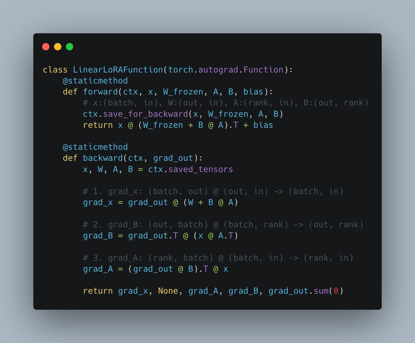
All of this means that training of relatively big models can be successfully done on even a single node. As long as the model weights fit in memory, we should be able to train MoE-style models with hundreds of billions of parameters. In full-model fine-tuning, storing the gradients and optimizer states balloons the memory footprint far beyond what a single node can handle, requiring multiple nodes, which significantly increases the training complexity. With the adoption of LoRA, training can be executed on a single node. With the adoption of LoRA, the training itself can be executed on a single node, while inference runs on another independent setup.
Economies of scale in inference
As the seasoned readers of our publication probably already know, LLM inference is primarily memory-bound, meaning that token throughput is mainly limited by the time it takes to load the model parameters into the GPU’s streaming multiprocessors (SMs) from GPU memory rather than by the time it takes to perform calculations within SMs. If the reader is unfamiliar with the concept of a roofline model and computation being compute-bound or memory-bound, we highly recommend our past article that introduces these concepts and explores them in detail in the context of LLM inference.
Being memory-bound has pretty straightforward implications. In order to decrease the cost of producing a token, we need to increase the number of tokens produced within a unit of time. If producing a token means mainly waiting to load the model parameters, we can load them once and use the same loaded parameters to serve multiple queries in a single batch.
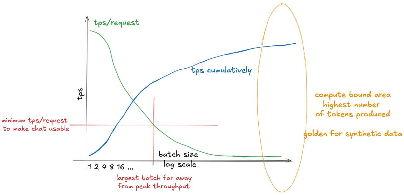
This increases the cumulative number of tokens produced sublinearly - throughput improves with batch size, but at a diminishing rate. As we increase the batch size, this comes at a cost: the speed individual users experience will decline over time, as demonstrated in Fig. 11. This is mostly due to the KV cache growing larger. As we increase the batch size, the KV cache starts to dominate the load time, and the improvements we observe diminish. However, as we increase the batch size, we saturate the available compute better, driving down the cost of producing an individual token, making it cheaper to serve.

This is even more relevant in the case of Mixture of Experts (MoE) models - the most popular architecture of powerful models as of November 2025,. As we wrote in our previous article on MoE inference:
During the decode phase, each token in the batch is activating only a small subset of parameters at every layer. This means that each request requires us to load a different part of the model, as demonstrated in Fig. 12. As the number of requests in a batch increases, a more and more substantial portion of the model will have to be loaded from global memory. The experts are chosen semi-stochastically1, so some of the tokens in the batch will be routed to the same expert. As we progressively increase the batch size, more and more experts will be shared by different requests. This means that at the larger batch sizes we will partially recreate the situation from the dense model - sharing the cost of model loading between multiple users. Unfortunately this means that we will need significantly more requests.
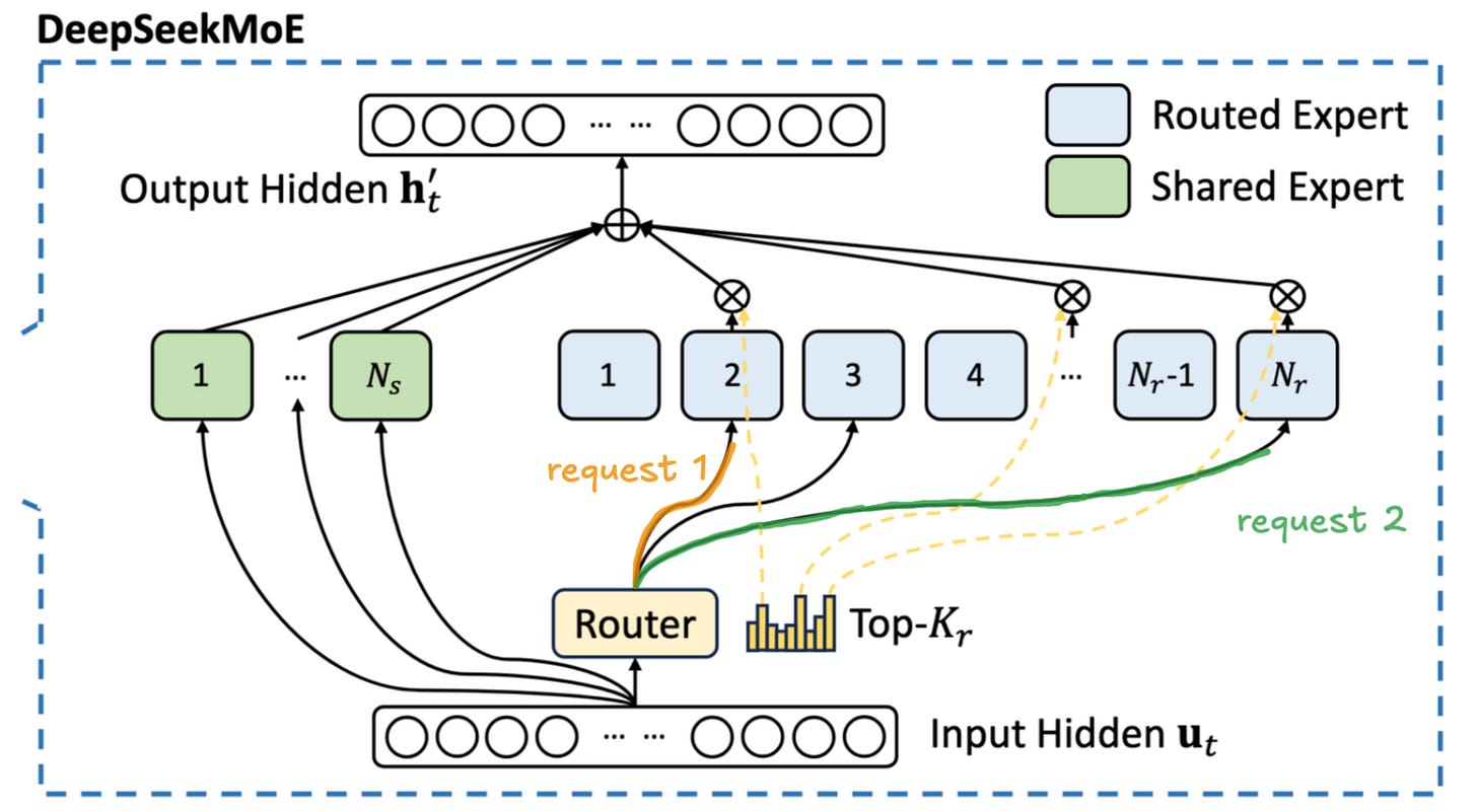
The main thing the reader should take away from this is that the key to good inference economics is large batches where we share the cost of loading the model weights between as many users as possible, achieving economies of scale of sorts.
This need for large batches might be problematic when we serve custom model fine-tunings. If we were to do full model fine-tuning for a model used by a particular user, this would be very hard to achieve unless we can guarantee massive demand. Some providers have this luxury - for example, Cursor Composer clearly has enough demand to achieve the necessary batch sizes - but if we are serving a model trained via RL by a smaller company to achieve superhuman performance at some niche task, it won’t be possible to find enough demand. Luckily for us, LoRA addresses this problem.
Throughout this text, we refer to the model on top of which we add LoRA adapters as the “base model.” This should not be confused with “base model” meaning a pre-trained model before instruction tuning. The base model can be any model on top of which we would run; e.g., for this model, Qwen3-30B-A3B-Instruct-2507 would be considered a base model.
When we are running LoRA-based model fine-tunings, it is much easier to achieve the necessary batch sizes. We can gather requests from multiple users, each using their own LoRA adapter. During the forward pass, we share the cost of loading the base model weights across multiple users. We still need to load the LoRA weights, which adds a little overhead, but as we showed in the previous section, LoRA adapters have a minimal memory footprint, and loading them is very fast.
This idea is called multi-tenancy and is the core technique that will enable the era of experience-style custom models to be served cost-efficiently. The inference provider will be able to serve thousands of adapters built on top of the same base model. During inference, we allocate a dedicated buffer to store the LoRA adapters of predefined shapes. Such a setup enables dynamically loading the adapters for which there is currently demand. If the particular adapter is not used at some point in time, it is offloaded from the buffer and replaced by another adapter requested by another user.
The exact details of how to implement this are quite complex and beyond the scope of this text, but the high-level is demonstrated in Figure 13. Multi-tenancy means we are able to dynamically load different adapters and share the cost of using the base model across multiple users, driving down the cost for individual users.
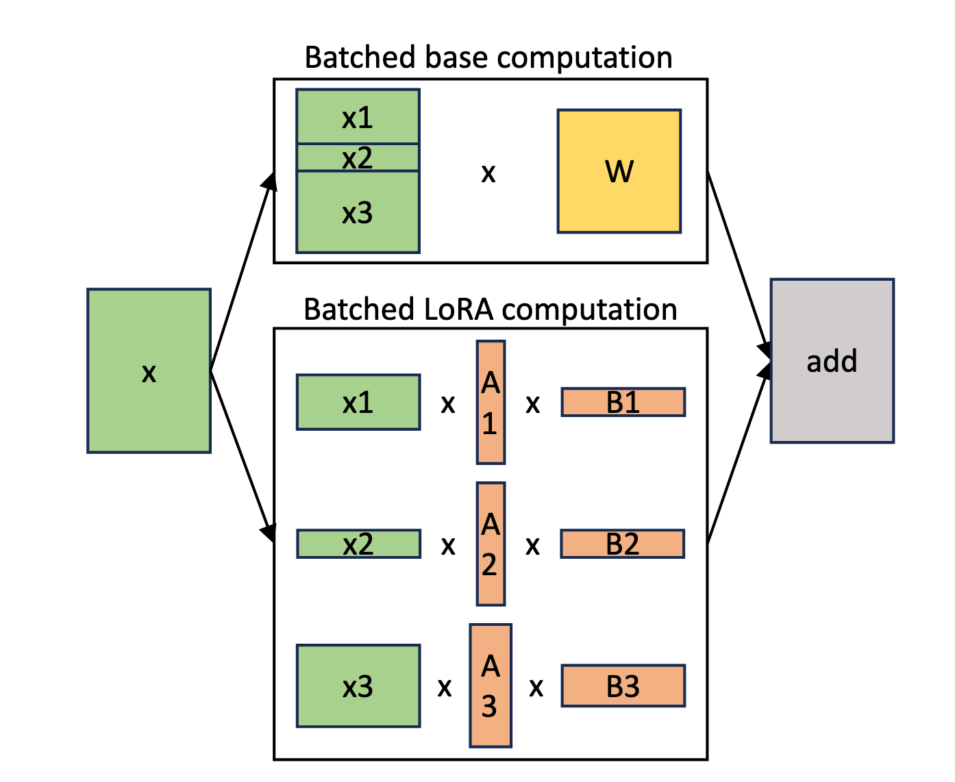
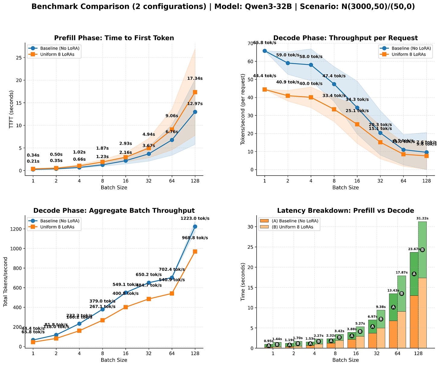
Modern inference engines such as SGLang and vLLM already have pretty sophisticated mechanisms to serve multiple LoRAs. In our experiments we were able to achieve ~85% of the baseline (no adapter) throughput when using LoRAs, as demonstrated in Fig. 14. Since the cost is a directly tied to the throughput achieved, this nicely shows how the cost of serving multiple adapters is only marginally higher than serving the base model alone.
Everything async and multi-turn
As we discussed before, in RL training we have two phases: training and generating rollouts. The workflow goes as follows:
We gather a set of prompts that we want to train the model on. This can be anything, from “write a Python program sorting numbers” to “solve this PhD-level math problem.” The only requirement is that we have some way to verify (or at least estimate) how well our model did on a particular problem.
We use the inference worker to produce the replies for a given prompt. Once the rollout is finished, we assign a reward to it. The exact reward formula is highly dependent on the problem; it can be anything from simple string matching (1 if matching, 0 if not) to sophisticated evaluations consisting of multiple steps such as compilation, running tests, comparing execution time, etc.
Once rewards are calculated, we can use them to calculate the advantages (as we showed in Fig. 5) and proceed to run the optimization step via GRPO as explained by the pseudocode in Fig. 4.
Once we run the optimization step and we have the new version of the model, we update the inference worker with the updated weights, and we repeat the cycle.
This is a high-level overview of an RL training pipeline. However, in practice, making it work is extremely challenging. One canonical problem is token lag. Token lag refers to the number of optimizer steps between the current policy (π_θ being trained) and the old policy (π_θ_old that generated the samples). We sample the rollouts using some policy. We grade the outputs, and then we proceed to training. Due to memory limitations, we train on small batches, consisting of a few rollouts - not on all rollouts at the same time. We update the policy π in each optimization step (on each minibatch). This means that as we calculate the next steps, the divergence between our current policy and the original policy from which we sampled the rollout widens.
In RL, this is traditionally measured through the Effective Sample Size, or ESS. When using off-policy RL, ESS measures how many samples from the current policy π_θ would yield equivalent performance to weighted samples from the sampling policy π_θ_old. The (normalized) ESS is defined as:
Where:
N is the sample size.
ESS ≈ 1.0 (100%): Perfect! Data is basically on-policy, all samples equally useful
ESS ≈ 0.1 (10%): Most samples are useless, a few dominate → high variance, unstable training
ESS is like asking, “Out of my 1000 samples, how many are actually informative vs. just noise?” If only a few samples have all the importance weight, you effectively have very few useful samples.
As we move away from the original policy, the token lag increases, as demonstrated in Fig. 15. This causes ESS to decrease, meaning our samples become progressively less useful for training.
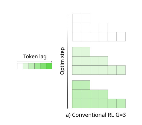
This is a major problem in RL - from the later samples we learn less and less. This naturally limits our sampling batch size. We can’t produce too many examples for the trainer, because they will not be very useful, as we’ve diverted too far from the sampling policy anyway. This limit in the batch size introduces another problem. Since inference is memory-bound, we want as large batches as possible to achieve high utilization and produce the maximum number of per second. Yet because of low ESS in samples coming later, we can’t effectively utilize these larger batches. This is very wasteful and limiting, substantially slowing down the training and driving up the costs.
To address this, nowadays most organizations are using some sort of Asynchronous RL. The concept is rather simple, as we demonstrate in Fig. 16. We operate three types of workers running concurrently: the training worker, the inference worker, the grading worker. They all run at the same time and communicate through queues.
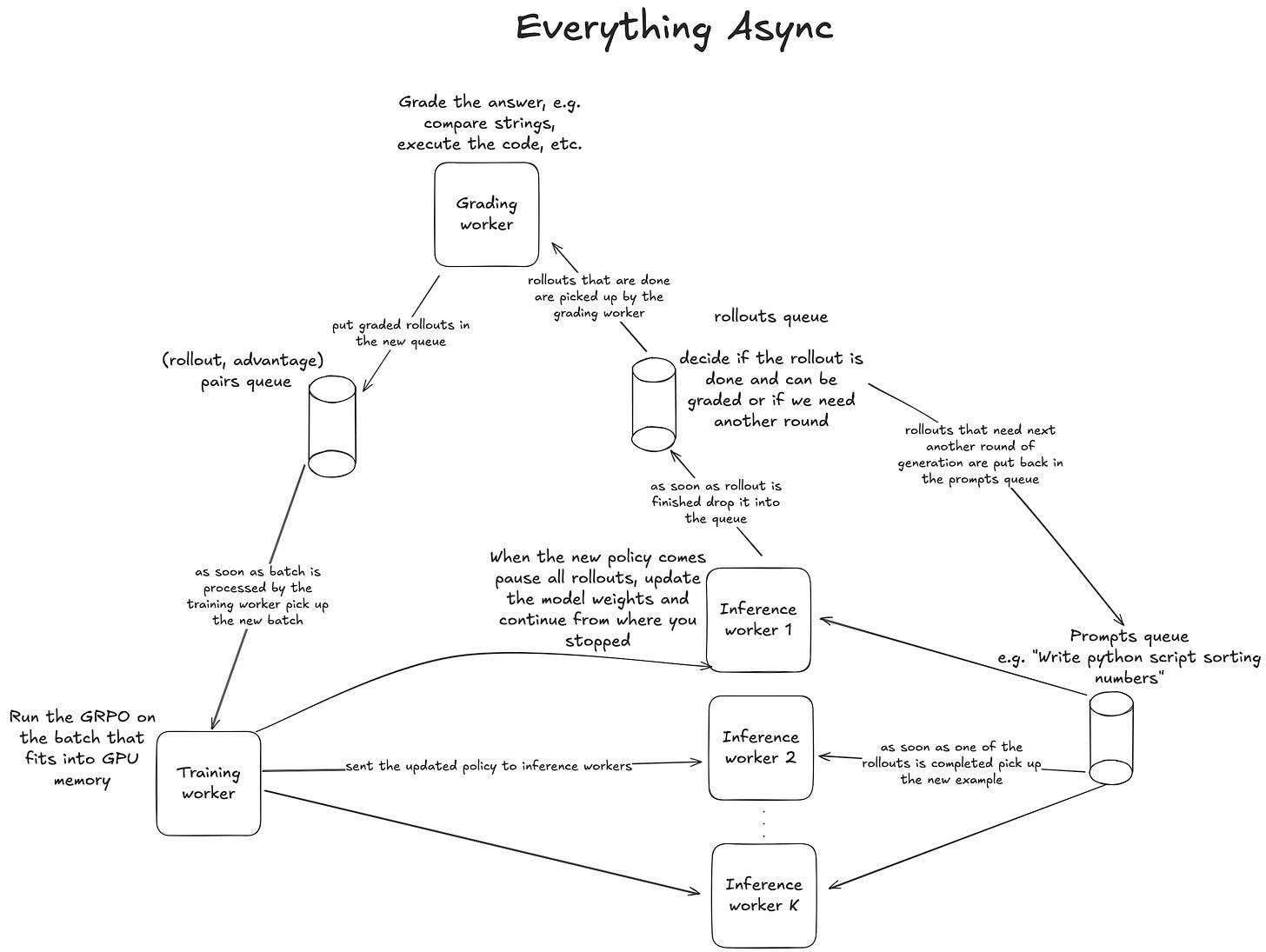
First, we have inference workers. They pick up prompts from the prompt queue and sample the rollouts, then they push the rollouts to the “completed rollout queue,” where they can be picked up by the grading worker. Depending on the problem, grading can either be very fast, e.g., for a simple string comparison, or take longer than generating the rollout itself, e.g., when it requires time-consuming compilation of a CUDA kernel. Ideally, we would like to scale the grading workers so that the overall throughput of the system is limited by the speed of the inference workers rather than by the grading workers, since the grading workers are usually CPU-bound - hence scaling them should be much cheaper than scaling the GPU-based inference.
After the rollout has been assigned a reward, we can proceed to calculate the advantage. In GRPO, advantage for rollout i is calculated as:
This means we can only calculate it after we have graded all rollouts for the same prompt. In Fig. 5, we demonstrated a simple example of this calculation.
Multi-turn interactions and tool usage add additional complexity to this pipeline. In multi-turn RL, instead of generating a single response, the model engages in back-and-forth exchanges, each turn building on previous context. The rollout now consists of multiple conversation turns, and the reward might only be assigned after the entire conversation concludes. For example: “Did the model successfully build a computer program I asked for across all turns?” or “The model made 6 guesses in WORDLE - did it guess the correct word in the end?”
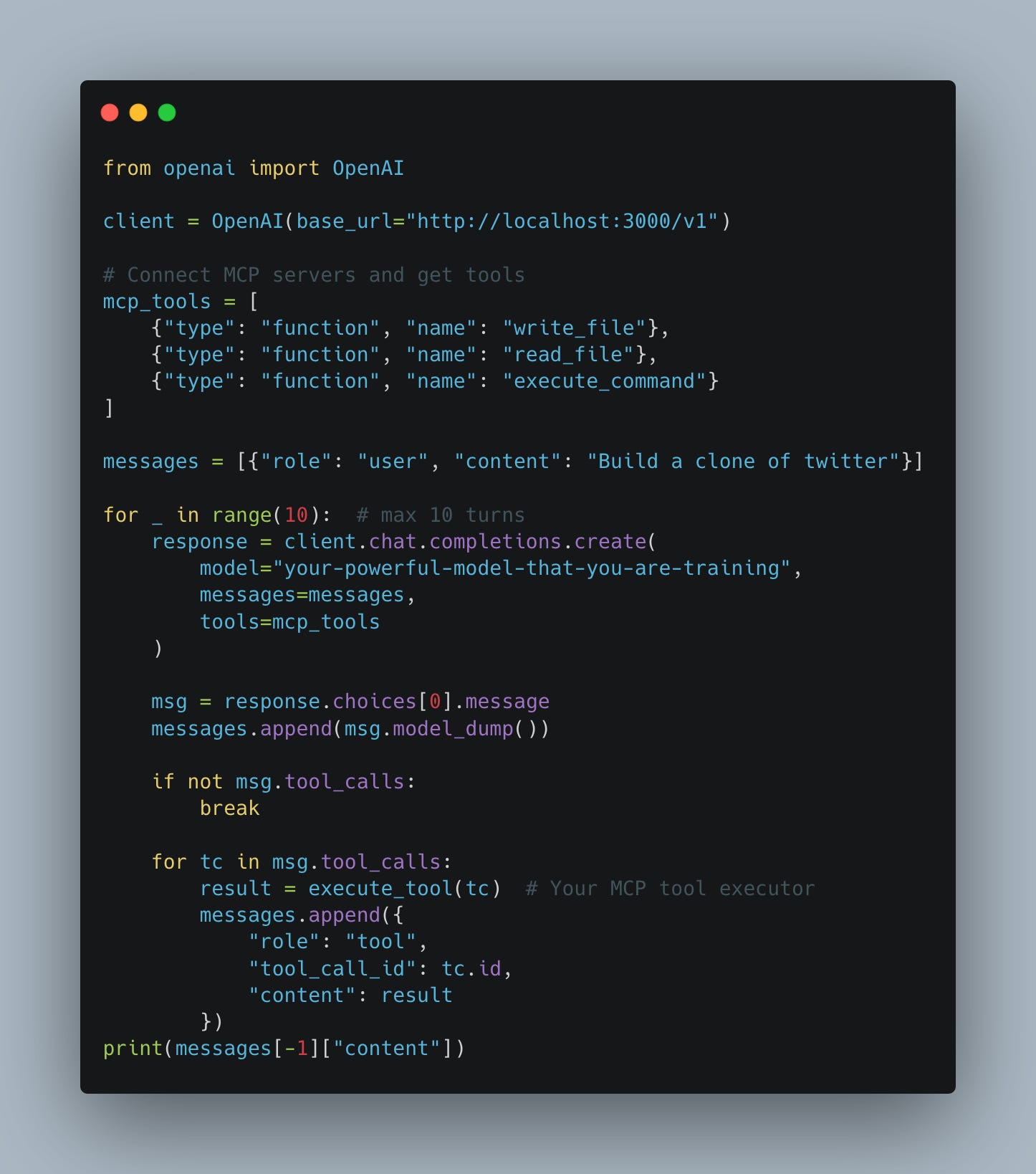
Additionally, modern RL setups often involve tool-calling, where the model can invoke external functions during generation, for example, as demonstrated in Fig. 3 in the context of Cursor Composer. The “conversation” might consist of model replies, feedback from the environment (e.g., “you did not guess correctly, try again”), and the results of function calls (e.g., what the Python interpreter returns). While there exist all sorts of sophisticated “agentic frameworks,” at the end of the day, an “agent” is just a loop: iterate over turns, pass context to the model, execute any tool calls, append results back to the context, and repeat. We provide a high-level example of such a system in Fig. 17.
Once we grade the examples, we can proceed to training and run an RL optimization step. The trainer worker requests batch size B examples from the graded examples queue. In practice we would most likely choose the biggest batch size that will fit into GPU memory. We calculate the RL loss (e.g. GRPO), run a single optimizer step, and send the updated weights to the inference workers.
Inference workers, when they get a weight update, briefly pause generation to update the model weights, and then continue from where they stopped. Crucially, the KV-cache is not recomputed, meaning it goes out of sync with the new weights - a misalignment that adds to the unintuitive nature of why this works at all. Consequently, a single rollout will be comprised of tokens sampled using various, continuously updated versions of the policy. It ensures that the token lag will be spread relatively evenly across all examples, as demonstrated in Fig. 18, not concentrated in the examples processed later in time by the training worker (as we saw in Fig. 15).
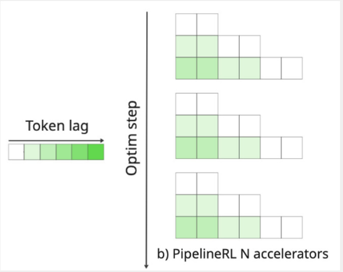
While it seems unintuitive that it works at all, it has been shown empirically that it performs remarkably well, learning different problems much faster than conventional RL. The key additional benefit of async RL is that it enables sustainably running larger batches and producing more tokens in the same amount of time, resulting in faster training through better hardware utilization.
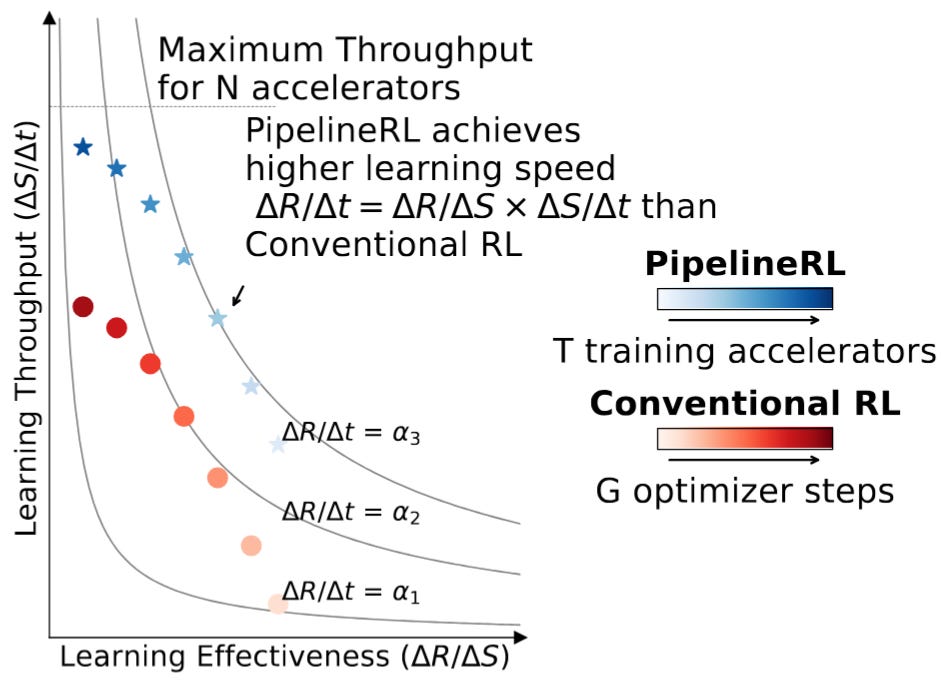
In RL the learning speed can be expressed as a simple product between how good our samples are at teaching the model the new task and the number of samples we process per unit of time.
Where:
Speed (ΔR/Δt): How fast does reward improve over time?
Effectiveness (ΔR/ΔS): How much does reward improve per sample? (data quality)
Throughput (ΔS/Δt): How many samples can we process per unit time? (computational efficiency)
In classic RL the batch size (throughput) was naturally limited - as over time the effectiveness of the samples was going down, to zero at some point, meaning that increasing the batch size provided no additional benefits. With Async RL the effectiveness is maintained for longer, and we can operate on substantially larger batches, driving up the throughput and increasing the learning speed as a result (see Fig. 19).
The best introduction to async RL the reader can find is “PipelineRL: Faster On-policy Reinforcement Learning for Long Sequence Generation.” We want to highlight this to the readers as a truly remarkable work! Very well written, with a great open-source implementation. We highly recommend the reader give it a read when they have time if they want to understand async RL concepts at a deeper level.
LoRA in RL
Both the training itself and rollout generation can greatly benefit from combining async RL with LoRA.
In model training, when we use LoRA, we don’t need to store the gradients and optimizer states for all the parameters. We just need to store the base model weights, gradients for small adapters (3-4 orders of magnitude smaller, as we showed earlier), and activations4. Since gradients and optimizer states are a substantial portion of the memory footprint during full model training, this means that when training using just the LoRA adapters we can massively increase the batch size. The memory footprint of activations will still scale linearly with the batch size, as will the FLOPs, but LoRA requires only about 2/3 of the FLOPs compared to full fine-tuning.
While the exact details depend on factors such as which base model we are using, where we apply LoRAs, and what the LoRA rank is, the key takeaway is that LoRAs enable us to run training at substantially larger batches due to massively reduced memory requirements for gradients and optimizer states. This means that the training worker can process rollouts from the inference workers faster. Since it processes rollouts faster, at some point the training worker will start to idle - there won’t be enough rollouts to consume. This means we can reassign the workers, moving some compute resources (GPUs) from training to inference, further accelerating the throughput. Now inference has more resources because training requires fewer, so we can produce more rollouts.
As we discussed in the previous section, running inference with LoRA adapters results in only minuscule performance degradation compared to the baseline (”without regret”). This has profound implications for the economics of rollout generation. It becomes technically feasible to combine rollout generation from multiple policies, each optimizing different reward functions, all built on top of the same base model within a single inference setup.
Inference is memory-bound, so throughput and utilization per GPU increase as we increase the batch size. If we combine multiple LoRA adapters, we can linearly scale the batch size, driving down the marginal cost of producing a token, decreasing the overall cost or enabling much larger scale on some fixed budget as a result.
This property can be extremely useful both for RFT and for full model fine-tuning. For we can use multiple policies and combine them into a single massive batch, fully utilizing the provided compute. Already today a number of companies, such as Thinking Machines or Weights and Biases, offer “RL as a service”-type of products, where clients can train their LoRA-based model fine-tunings running on top of open-source models. Using a single inference setup for multiple clients can be an important axis of cost optimization for these providers, driving down the costs and increasing the margin (assuming there is enough demand, which remains unclear as of today).
What is less obvious is that this ability to combine multiple independent policies into a single inference setup can also be valuable for organizations training universal foundation models. Often when training the model, initially the team would train a few different, independent models, each optimizing a different reward function. After we have a few trained models with good performance on these independent tasks, we would apply some sort of model distillation technique to bring all of these capabilities into the single final model. For example in the report for DeepSeek v3.2 we read:
For each task, we initially develop a specialized model dedicated exclusively to that particular domain, with all specialist models being fine-tuned from the same pre-trained DeepSeek-V3.2 base checkpoint. In addition to writing tasks and general question-answering, our framework encompasses five specialized domains: mathematics, competitive programming, general logical reasoning, agentic coding, and agentic search. Each specialist is trained with large-scale Reinforcement Learning (RL) computing. Furthermore, we employ different models to generate training data for long chain-of-thought reasoning (thinking mode) and direct response generation (non-thinking mode). Once the specialist models are prepared, they are used to produce the domain-specific data for the final checkpoint
If the DeepSeek team were to train these models through LoRA adapters (remember “no regret”), they could combine prompts for different models and run them on top of a single inference setup. This would be much, much more efficient than running five separate setups.
The mental picture we hope the reader takes away from reading this article is the visualization shown in Fig. 20. To increase the throughput of token generation, we need to run very large batches. This comes at a tradeoff - any single generation will be relatively slow, but this doesn’t matter much for RL rollout generation, since we don’t have human users impatiently waiting for a response to appear. All we care about is producing as many tokens as possible given a hardware budget, and here we achieve just that.
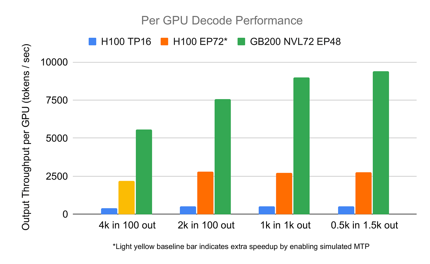
The ability to run larger batches is especially relevant for large-scale MoE models, such as DeepSeek. As we elaborated in detail in our previous text on “MoE Inference Economics from First Principles,” this class of models, due to their sparse computation patterns, greatly benefits from a high concentration of GPU resources in a single setup. If the inference provider is capable of running a setup spanning multiple nodes, the performance per GPU will be significantly improved compared to a setup spanning one or two nodes, as demonstrated in Fig. 21. This means that if our training setup allows for larger batches, we can combine multiple nodes, increasing the performance per GPU. All these factors compound, resulting in substantially faster and cheaper training of RL models.
Additional benefit of the minuscule memory footprint of LoRAs comes up during the policy update when the training worker sends the updated policy to the inference workers. Because the LoRA weights are so small, sending them from one worker to another is very quick. There is little to no overhead - updates are fast and inference GPUs aren’t left idling during synchronization.
Intelligence markets through RFT
In this text we tried to introduce the technical details that will underpin the “experience economy.” We argue that policy gradient optimization methods, such as GRPO, are very information sparse, providing only log(N) bits per rollout, where N is the reward granularity. Because of this, the data learned by the model can be efficiently encoded in very few parameters. We can do this parameter-efficient fine-tuning technique, such as LoRA, without any penalty (“no regret”) to the model performance compared to the full model fine-tuning.
LoRA makes training substantially cheaper because we don’t need to store the optimizer states nor gradients for the parameters. Hence, on the fixed hardware budget, we can run substantially larger batches, increasing the speed of training. In the context of RL, this means that we can allocate fewer resources for training and more towards inference workers, driving up the data generation speed.
LoRA unlocks the ability to scale the batch size, which plays nicely with ideas of AsyncRL - the leading paradigm of doing RL in 2025. In AsyncRL different tokens in a single rollout are sampled using multiple continuously updated policies. Empirically it has been shown to improve the end-to-end performance as the token lag is spread more evenly throughout the samples.
Because competing with the foundation’s general-purpose model is so challenging and capital intensive, focusing on model specialization seems like a promising path for less resourceful organizations. The biggest of the recent releases in this domain was the introduction of Tinker by Thinking Machines, where they enable organizations to run RL workloads. The distributed training is abstracted away and handled by Thiky. The user of the API has to only focus on reward modeling. Pricing is divided into inference parts (prefill + sampling) and training parts (see Fig. 22).
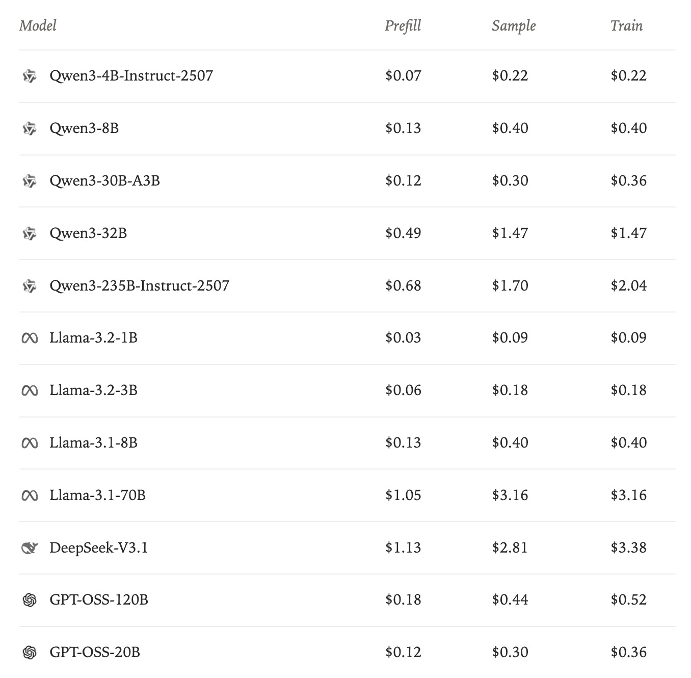
The RFT-type services, in our opinion, offer a great opportunity for NeoClouds to increase the margins on compute in smaller clusters. RFT is specifically well positioned to utilize the smaller clusters (a few hundred nodes). Since the memory requirements are so significantly reduced, and we have only 2/3rds of the FLOPs of full-model fine-tuning, training can be conducted on substantially reduced resources, potentially even within a single H100 node for models of +200B parameters. Moreover, using multi-tenancy, it is possible to gather requests from multiple users into a single large batch, further increasing the cost competitiveness.
This has great potential to improve the profit margins on the underutilized compute resources gathered in the smaller datacenter - the compute that up until now was of limited potential, as it was not possible to run larger training runs of it - thing that offers the highest margins.
You can see that NeoClouds are already interested in this direction. E.g., in September 2025, CoreWeave acquired one of the startups pioneering RFT - OpenPipe. CoreWeave also acquired Weights and Biases, which also offers an RL-as-a-service-type product, since October 2025.
The big question is whether there is actually a market for RFT - if there is any point in developing these capabilities, or will the smart models be able to just “figure it out” in context, as they get more and more intelligent? This we can’t answer. What can be argued is that as of today it is not the case; there are clearly moats to be built in this fashion. There are some capabilities that are inherently “not there” in cloud models.
Two good examples are the model’s ability for persuasion in a particular domain. The best example here is the AdLlama paper from Meta. Researchers first train a reward model based on the user preference data. The reward model is able to estimate which headline will “click” with users and which will be ignored. Then the said model was used to optimize Llama 2 (it took them a while to publish this paper) using PPO, so it is more likely to produce more persuasive outcomes. The high-level overview we present in Figure 23.
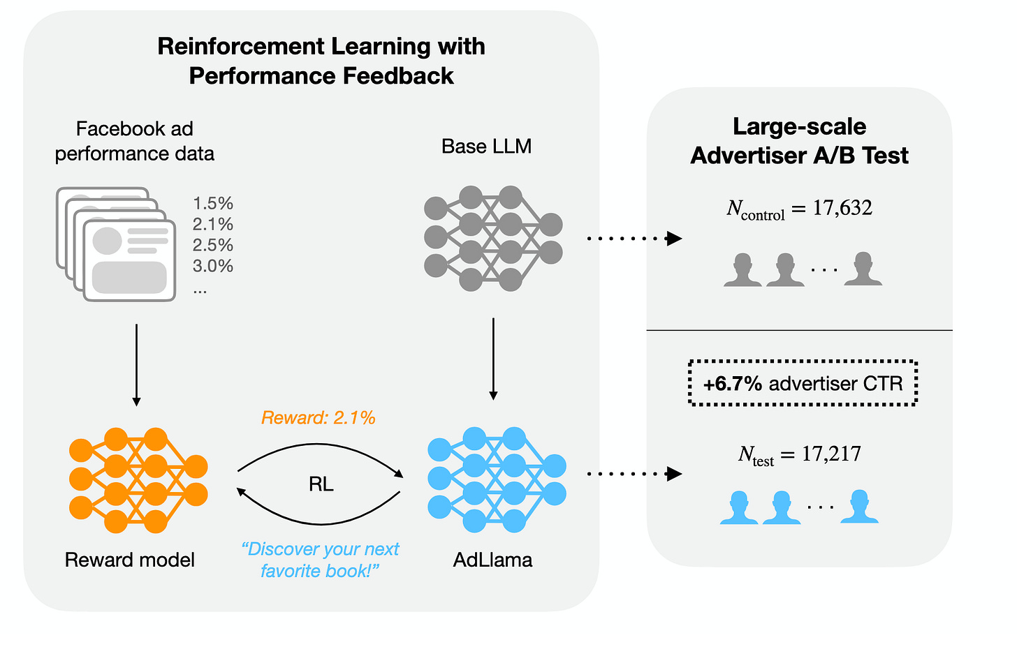
Data on how to best persuade the users of Facebook are clearly not available directly on the Common Crawl. It requires a pretty sophisticated data-gathering mechanism that also can be further refined by providing specific demographic data (e.g., user age, sex, embedding of preferences, etc.) to make the reward model more accurate. A language model optimized using such a reward model is most likely to be much, much better at persuasion than off-the-shelf GPT, though it is fair to say that in the future, as models get more intelligent, the ability to persuade might be just “baked” in them, since they already have a pretty high emotional intelligence.
Another example of successful RFT is building custom deep research systems. The most successful deep research models today are already trained today with RL reward modeling. Training is organized as follows: we ask a question, the model does a number of function calls, web searches, and coding, and maybe searches through third-party tools, and after a number of turns produces a final answer (like in the simple agent loop we introduced in Fig. 17), and the system provides a reward based on how well the model did on this task.
Every company has slightly different data; some use Confluence, others some obscure SAP system written in the 1980s, and others just a continuously updated Excel sheet. It can be argued that this might be too diverse for an out-of-the-box model to be able to search through it successfully, and to build a competitive advantage, companies should be training models that get better at utilizing THEIR data over time. Whether the overhead of this will be too substantial, building good environments is challenging and requires some expertise, or it will be worth it remains to be seen as of now.
The major challenge of RFT is that it requires building custom environments for every problem to be solved, which is inherently not scalable. LLMs can potentially help here, in aiding humans in building these environments, but in our experience, as of late 2025, in zero-shot fashion setups, LLMs exhibit a pretty poor performance when it comes to reward modeling, requiring substantial supervision from humans. Not surprisingly, most of the companies in this space right now focus on building “picks and shovels” of RFT, be it the fine-tuning platforms like we discussed for Thinking Machines or building the environments hub like Prime Intellect.
While these make it easier to iterate on custom models, the main problem of making custom models useful - how to scale environment building and reward modeling remains unsolved. The training foundations are there - the unknown remains the path to scaling.
Acknowledgments
Thanks to each of you for giving me feedback. Lukas (absolute 🐐) for having an insane eye for detail and correcting me on errors small and not so small. Pieter for giving it a first read and pointing out networking advantages, Jordan for discussing the NeoCloud perspective with me. Vedant (big win for Mistral) for his comments on ICL and era of experience. Szymon and Felix for providing me with small suggestions on how to direct this text, and to Felix for discussing with me the token lag problem. Andreas for challenging the 1 bit idea.
@online{tensoreconomics2025aiinfraineraofexperince,
  author = {Piotr Mazurek},
  title = {AI infrastructure in the "Era of experience"},
  url = {https://www.tensoreconomics.com/p/ai-infrastructure-in-the-era-of-experience},
  urldate = {2025-11-16},
  year = {2025},
  month = {November},
  publisher = {Substack}
}At tensoreconomics we doubt this is actually the case as of today. We believe that there still remains a gap between open-source models and frontier models from Anthropic, OpenAI and most recently Google. The gap is poorly captured by the existing benchmarks, but it is clearly showed by the consumer interest. People just don’t use these free models, but pay for Claude, GPT or Gemini subscriptions.
E.g. facebook/opt-125m models have 4M monthly downloads as of November 2025, even though no one is using them. It is most likely caused by them being the default model used in vllm documentation.
There are limits to this analogy. For example, until recently the Chinese model providers were unable to secure enough compute capacity to serve their models competitively. Users wanting to use Chinese models typically access them through Western inference providers, such as Together or Fireworks. This is in clear contrast to the traditional model where Western companies dominated “IP” and Chinese companies dominated manufacturing; here the dynamic is reversed.
The exact footprint of activations stored is highly dependent on the activations checkpointing strategy.

very well written, and super interesting
God’s work!! I hope you continue writing.